Problems before Sentiment Analysis
In the first Blog, we conducted data collection, data observation, data preprocessing and wold cloud. Before we gave scores to FOMC statements, we found that the previous cleaned statements had better be several short sentences instead of single words and long sentences. Besides, we found that some useless sentences, such as the ones beginning with "please email" or "voting monetary", appeared a lot. In the case, we further cleaned the data.
def preprocess_text(text):
    # transfer to lowercase
    text = text.lower()
    #Remove names
    nlp = spacy.load('en_core_web_sm')
    doc = nlp(text)
    text = ' '.join([token.text for token in doc if token.ent_type_ != 'PERSON'])
    #Remove URLs
    text = re.sub(r'http\S+|www\S+|https\S+',' ',text)
    #Remove email address
    text = re.sub('([\w\.\-\_]+@[\w\.\-\_]+)',' ',text)
    #Remove phone numbers
    text = re.sub('(\d+)',' ',text)
    # Remove punctuation (keep sentence segmentation symbols)
    text = re.sub(r'[^\w\s,;:.?!]', '', text)
    sentences = re.split(r'[;,:.?!]', text)
    # token, stop words, remove specific sentences
    processed_sentences = []
    less4word=[]
    joinword=''
    for sentence in sentences:
        j=sentence.split(' ')
        tokens = word_tokenize(sentence)
        processed_tokens = [lemmatizer.lemmatize(word) for word in tokens if word not in stop_words]
        processed_sentence = ' '.join(processed_tokens)
        if not processed_sentence.startswith('please email') and not processed_sentence.startswith('voting monetary'):  # remove specific sentences
            processed_sentences.append(processed_sentence)
    while '' in processed_sentences:  #ensure no empty list
        processed_sentences.remove('')
    return processed_sentences
Sentiment Analysis
We performed sentiment analysis using the TextBlob library and the LM dictionary from pysentiment2. TextBlob is a powerful NLP library that offers various functionalities, including sentiment analysis. The default dictionary of TextBlob is a general dictionary from pattern. The following code was used to calculate the sentiment scores of the sentence:
score = TextBlob(sentence).polarity
Since we can customize the analyzer of TextBlob, we also utilized a pre-trained Naïve Bayes analyzer from NLTK to perform machine learning. Please note that if you try to switch to the NaiveBayesAnalyzer directly as the following code, TextBlob would be extremely slow:
Score = TextBlob(sentence, Analyzer = NaiveBayesAnalyzer()).sentiment.p_pos
The reason is that Textblob will train the analyzer internally before each run. To address this, we use Blobber from TextBlob to avoid training before each run:
from textblob import Blobber
from textblob.sentiments import NaiveBayesAnalyzer
tbnb = Blobber(analyzer=NaiveBayesAnalyzer())
score = tbnb(sentence).sentiment.p_pos
Another thing to mention, please use tbnb(sentence).sentiment.p_pos when you use the NaiveBayesAnalyzer instead of tbnb(sentence).polarity otherwise NaiveBayesAnalyzer would not work and you will get the same result as the default TextBlob. Additionally, we incorporated the LM dictionary, which is a famous dictionary in finance. It extends a common baseline dictionary to include words appearing in financial documents such as 10-K fillings and earning calls. For this analysis, we focused on calculating the polarity of the word. The first challenge we faced was there were so many place and position names in the statement. As they were useless for sentiment analysis, we excluded them from the calculations.
def remove_short_sentences(df):
    """
    Remove sentences with length less than 3
    """
    for i in range(len(df['content'])):
        df['content'][i] = [sentence for sentence in df['content'][i] if len(nltk.word_tokenize(sentence)) > 3]
return df
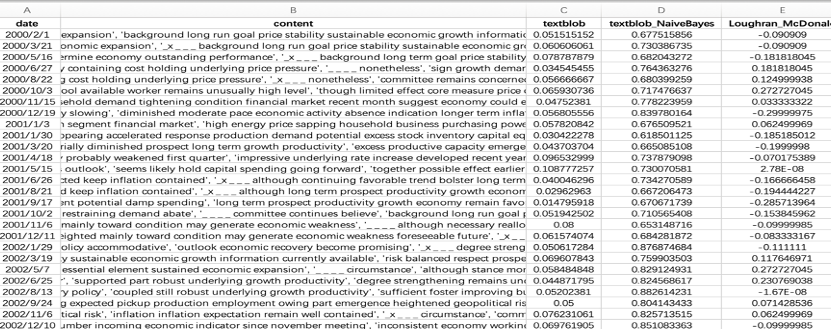
To determine the sentiment score of each statement, we computed their sentences’ scores first and then took the average. The deliverables here showcase our data structure. The first two column are the date and content of each statement. The third to fifth column displayed the sentiment scores we calculated.
Statistical Analysis
We only choose the sentiment score calculated using Loughran and McDonald dictionary method in this statistical analysis, which range is from -1 to 1. We construct senti_ploar column to see whether the score is positive or negative and event_indicator column to see whether the statement is released at the date. Then merge the factor data with daily 10-year US government bond yield (TNX). One thing should be noticed here is that the Adj Close data of TNX we download from Yahoo Finance is exactly the return rather than price. The other problem is that we do not have daily score data, because they only happen in specific date. Therefore, we set 0 for missing values for those missing data days, then lag these factor data and run linear regression on the daily 10-year government bond yield. Therefore, we could get the beta of sentiment score to see whether it can affect the US government bond yield.
diff_data['yield_diff'] = diff_data[yield_name].diff()
shift_lag = 1
diff_data['score_lag'] = diff_data[score_name].shift(shift_lag)
diff_data['polar_lag'] = diff_data['senti_polar'].shift(shift_lag)
diff_data['event_lag'] = diff_data['event_indicator'].shift(shift_lag)
diff_data = diff_data.dropna().reset_index(drop=True)

X_name = ['score_lag','polar_lag','event_lag']
X = sm.add_constant(diff_data[X_name])
y = diff_data[yield_name]
model = sm.OLS(y, X).fit()
However, we may wonder that set a window period may help to improve the estimation. Therefore, we set event window from 5 calendar days before the release of statement to 5 calendar days after. Moreover, during the presentation, the course instructor suggested that we should consider about trading strategy. Therefore, we find iShares U.S. Treasury Bond ETF (GOVT), which investing at least 90% of its asset in US Treasury securities. We believe this ETF may have homogonous change with the change of US Treasury bonds. Then we run regression by only sentiment scores on the 10-year US Treasury bonds and ETF respectively. We only get significant beta of sentiment scores when run regression on the log return of ETF with event window. Furthermore, we run regression on the standard deviation of their window return. The result gives us significant beta, which indicates that sentiment score can bring effects to the volatility of both TNX and GOVT.
cum_abnormal = sum(df_merge[yield_name] - df_merge['yield_predict'])
idx_event = slice_event[slice_event['event_indicator']==1].index[0]
slice_before = slice_event.iloc[:idx_event+1,:]
slice_after = slice_event.iloc[idx_event+1:,:]
twoperiods_diff = slice_after['log_ret'].sum() - slice_before['log_ret'].sum() # difference of log ret of ETF on two periods
yield_std = slice_event[yield_name].std()
logret_std = slice_event['log_ret'].std()
df_temp = df_merge[df_merge['date']==date].reset_index(drop=True).drop([yield_name,'yield_predict'],axis=1)
df_temp['cum_abnormal'] = cum_abnormal
df_temp['twoperiods_diff'] = twoperiods_diff
df_temp['twoyields_diff'] = twoyields_diff
df_temp['yield_std']=yield_std
df_temp['logret_std']=logret_std
df_abnormal = pd.concat([df_abnormal,df_temp]).reset_index(drop=True)

X_name = [score_name] #,'event_indicator','senti_polar' ,'FFR','FG','LSAP'
X = sm.add_constant(df_abnormal[X_name])
y = df_abnormal['yield_std']#'cum_abnormal' 'twoperiods_diff' 'logret_std'
model = sm.OLS(y, X).fit()
print(model.summary())
Then, a problem of one factor analysis is lack of other factors' combination, so we tried to find some other factors which can be combined to discuss. We first look through the blog of previous year which is related to FOMC documents, they considered about some macroeconomics effects such as GDP, while they did not state clearly where they obtained the data. Due to the limitation of data source, we then decide to look for other factors. Gorodnichenko et al.(2023) used factors FFR, FG, LSAP investigated by Swanson (2021) to observe how voice tone of press conference after FOMC meeting will affect the bond market performance. We try to use these factors in our analysis process to see whether they can help. Unfortunately, the answer is no! Even though some factors have significant beta, but our sentiment scores become insignificant in this case. This may be because sentiment score is explained by these factors.
Limitations
-
Methods of Sentiment Scores: Lack of Contextual and Emotional Depth - Relying on dictionaries for sentiment analysis may not only miss the contextual meaning behind words but also overlook the emotional tone or intensity conveyed. Financial texts, especially those from institutions like the FOMC, often use nuanced language that can have a substantial impact on market interpretation and reaction. The emotional valence attached to certain terms or phrases could significantly influence investor sentiment and market dynamics, which dictionary-based methods may fail to capture.
-
Temporal Dynamics Ignored: The current analysis may not adequately account for the temporal dynamics between FOMC statement releases and changes in bond yields. The impact of statements on yields could vary over time, influenced by external economic events, market sentiment, or changes in monetary policy effectiveness.
-
Linear Models Limitation: If the study primarily relies on linear regression models, this could be a significant limitation. Financial markets are complex and influenced by a multitude of non-linear relationships. Linear models might not capture these complexities adequately, potentially oversimplifying the analysis and leading to inaccurate conclusions.
-
Overlooked Semantic Nuances:** Even with advanced text preprocessing, the sentiment analysis could miss out on semantic nuances such as irony, sarcasm, or technical jargon specific to financial contexts. This limitation could lead to misinterpretation of the sentiment conveyed in FOMC statements.
By addressing these limitations, the analysis could achieve a more nuanced and accurate understanding of how FOMC statements' sentiments affect government bond yields. We will give detailed suggestions for limitations in the final report.