By Group "Professional Team"
Our mission is to forecast interest rate trends based on FOMC speeches. This blog is mainly talking about the code part and problems we meet.
Data Collection
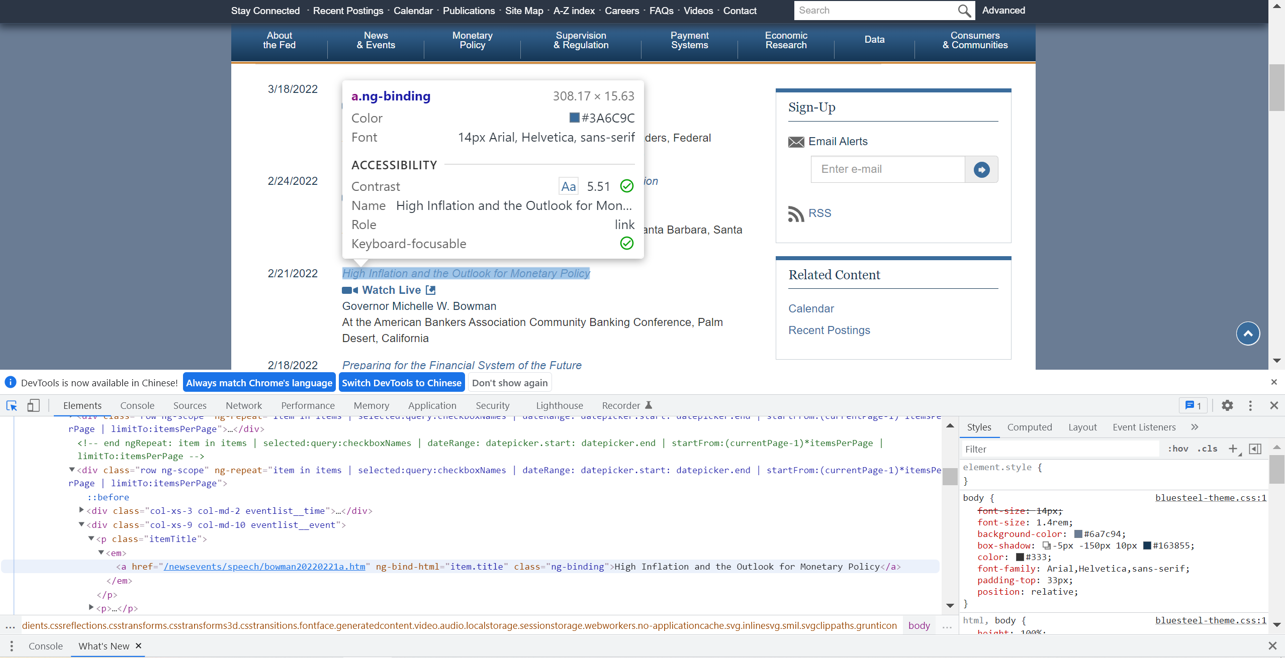
In the beginning, enter FOMC's official website. When we wanted to go to the next page, the website's URL didn't change, which meant that this page was a dynamic webpage. However, the web page's structure seemed simple, which was good news for us since it meant it was easy to scrape!
First, just press F12 to open DEVtools, locate the lecture's headline, then it would show us the lecture's URL. Copy its XPATH and use Selenium's find_element_by_xpath function then we could get the lecture URLs from the whole page. Then we needed to locate the "Next" button. Here we met a problem. Because every time we went to a different page, the"Next" button would change its position. So here we used Selenium's another function find_element_by_link_text.click()("Next"). It worked!
Here is the code for getting all lecture's URLs.
url=[]
for page in range(1,47):
    if page!=46:
        for x in range(1,21):
            url.append(driver.find_element_by_xpath('//*[@id="article"]/div[1]/div['+str(x)+']/div[2]/p[1]/em/a').get_attribute('href'))
        driver.find_element_by_link_text("Next").click()
    else:
        for x in range(1,16):
            url.append(driver.find_element_by_xpath('//*[@id="article"]/div[1]/div['+str(x)+']/div[2]/p[1]/em/a').get_attribute('href'))
Second, we went through all URLs, located the title, date, speaker, location and content. Here we used XPATH. Another problem happened.
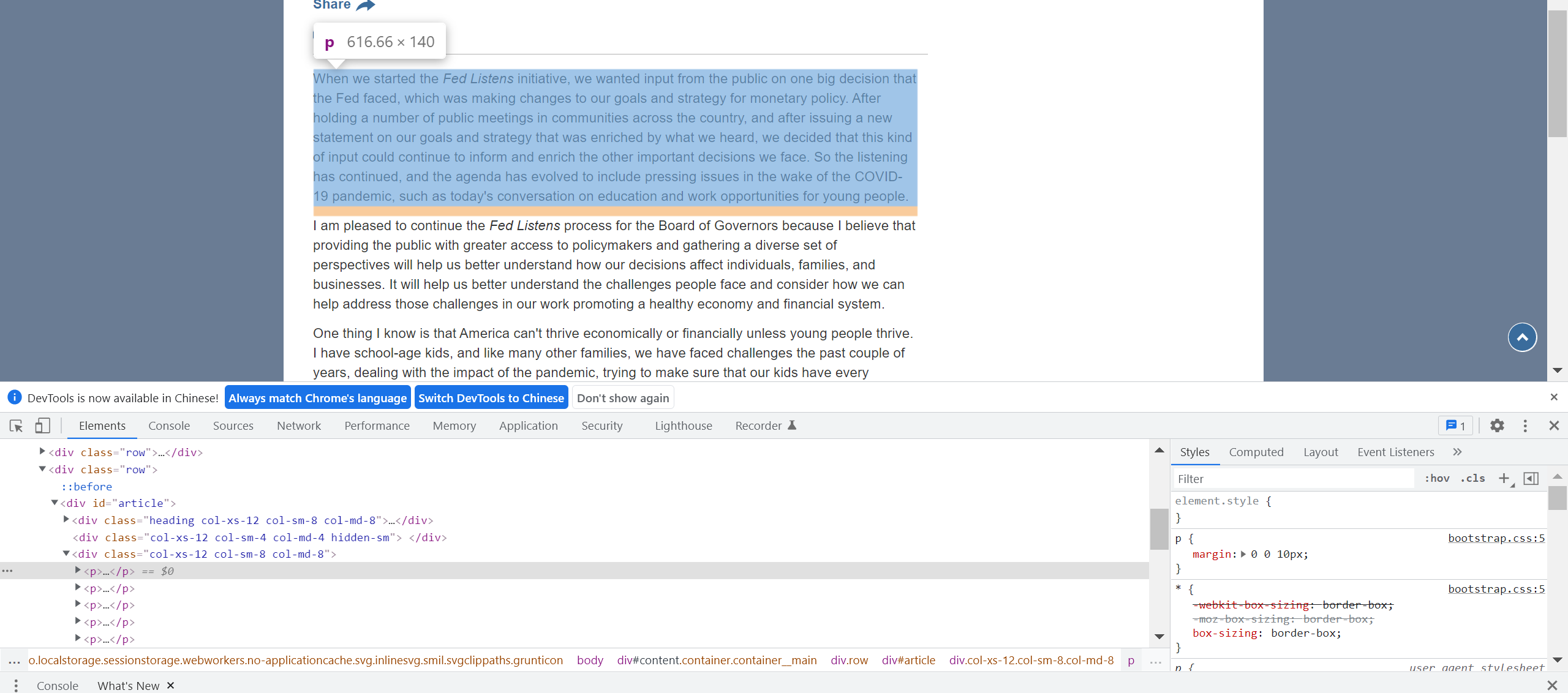
If we simply click the article, it was only able to locate one paragraph. The solution is to locate its parent node!
Finally, we got 915 speeches from 31 lecturers. The period was from January 18, 2006 to February 24, 2022.
Text Preprocessing
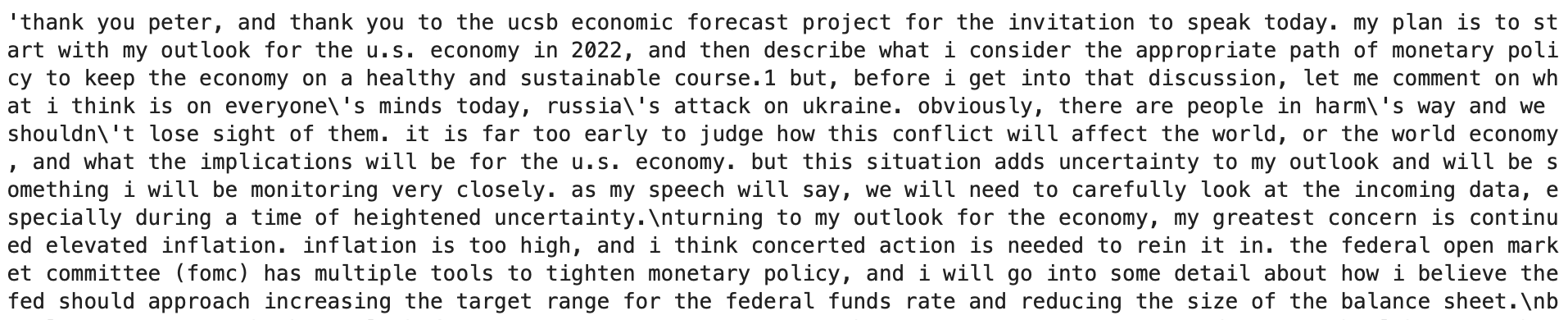
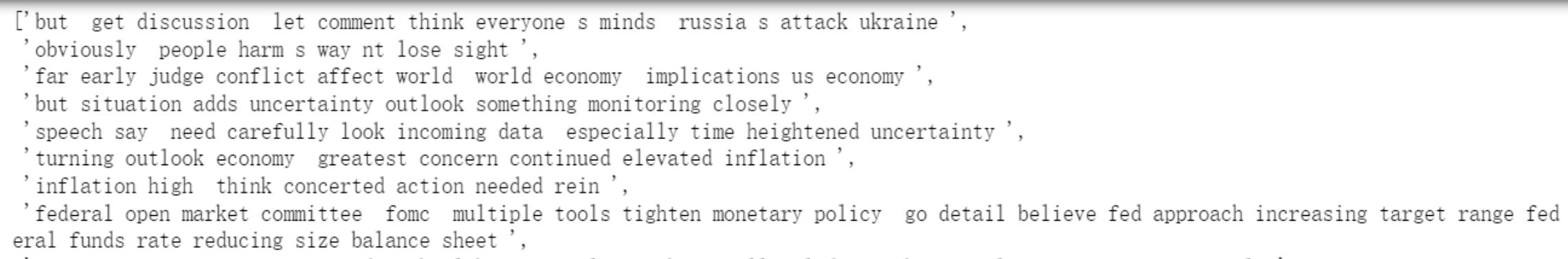
After scraping the information we needed from the website, we took out the speech content from the dataframe we created and made the lecture content in lower case for further processing. A speech example is showed below:
Then we defined some stopwords which were not important to analyze the sentiment in the lecture, like some prepositions, auxiliary verbs and some common words for the speech's opening. Additionally, since there were usually dates and numbers mentioned in the speech but difficult to confirm the connection between them in the text analysis, we also chose to delete them by using the datetime list downloaded from Github.
#Defining set containing all stopwords in English.
stopwordlist = ['a', 'about', 'above', 'after', 'again', 'ain', 'all', 'am', 'an',
             'and','any','are', 'as', 'at', 'be', 'because', 'been', 'before',
             'being', 'below', 'between','both', 'by', 'can', 'd', 'did', 'do',
             'does', 'doing', 'down', 'during', 'each','few', 'for', 'from',
             'further', 'had', 'has', 'have', 'having', 'he', 'her', 'here',
             'hers', 'herself', 'him', 'himself', 'his', 'how', 'i', 'if', 'in',
             'into','is', 'it', 'its', 'itself', 'just', 'll', 'm', 'ma',
             'me', 'more', 'most','my', 'myself', 'now', 'o', 'of', 'on', 'once',
             'only', 'or', 'other', 'our', 'ours','ourselves', 'out', 'own', 're',
            's', 'same', 'she', "shes", 'should', "shouldve",'so', 'some', 'such',
             't', 'than', 'that', "thatll", 'the', 'their', 'theirs', 'them',
             'themselves', 'then', 'there', 'these', 'they', 'this', 'those',
             'through', 'to', 'too','under', 'until', 'up', 've', 'very', 'was',
             'we', 'were', 'what', 'when', 'where','which','while', 'who', 'whom',
             'why', 'will', 'with', 'won', 'y', 'you', "youd","youll", "youre",
             "youve", 'your', 'yours', 'yourself', 'yourselves','thank','would',
                'like','speak','great','honor','today','$']

stoplist=[]
with open(r"pysentiment-master\pysentiment\static\DatesandNumbers.txt", "r") as f:
    for line in f.readlines():
            line = line.strip('\n')
            stoplist.append(line.lower())

stopwordlist=stopwordlist+stoplist

#Cleaning and removing the above stop words list from the lecture text
STOPWORDS = set(stopwordlist)
def cleaning_stopwords(text):
    return " ".join([word for word in nltk.word_tokenize(text) if word not in STOPWORDS ])
For further cleaning, we removed the references of the lecture posted at the end of each lecture and some additional URLs in the lecture content.
#Cleaning and removing URL’s
def cleaning_URLs(data):
    return re.sub('((www.[^s]+)|(https?://[^s]+))',' ',data)

#Cleaning and removing reference
def cleaning_references(text):
    return text.split("\n1")[0]
df1['content'] = df1['content'].apply(lambda x: cleaning_references(x))
df1['content'] = df1['content'].apply(lambda text: cleaning_stopwords(text))
df1['content'] = df1['content'].apply(lambda x: cleaning_URLs(x))
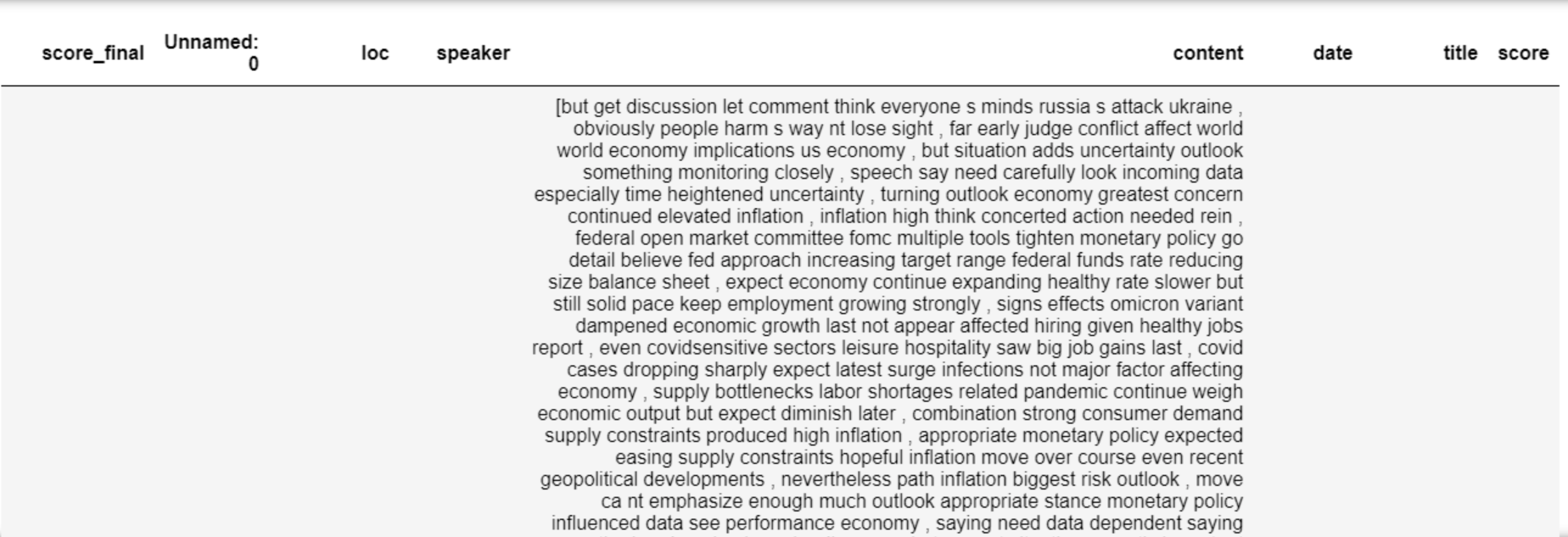
After these steps, the new lecture content is showed below:
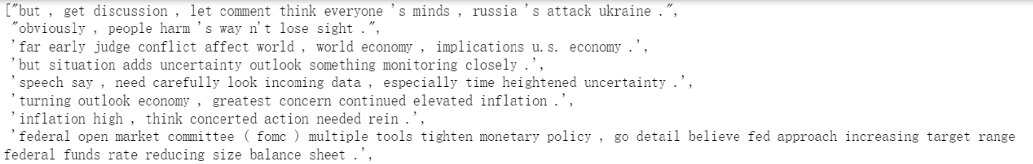
Considering the entire lecture content was complex and scoring its sentiment might be inaccurate or difficult. So we splited each lecture into several sentences in a tokenized way, and then deleted punctuations in each sentence.
Additionally, in the case of pretty short sentences, less information and extreme emotion might be reflected, which was another issue we needed to pay attention to when using the Loughran and McDonald's dictionary. So we deleted the sentences with words less than 8.
#Split the lecture into sentences
df1['content']=df1['content'].apply(lambda x: nltk.sent_tokenize(x))

less8=[]
for i in range(len(df1['content'])):
    df1['content'][i]=df1['content'][i][2::]
    less8.extend(list(filter(lambda x: len(nltk.word_tokenize(x))<8, df1['content'][i])))
    df1['content'][i]=list(filter(lambda x: len(nltk.word_tokenize(x))>=8, df1['content'][i])) # delete sentence that length <8
Word Cloud
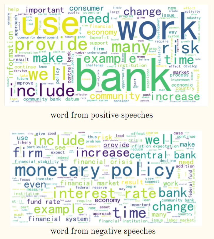
Here we built word clouds mainly based on former preprocessed text. We classified words into two categories. One was the words from positive lectures, one was the words from negative lectures. Since some phrases like "central bank", the word"central" and "bank" sometimes occurred together, we also made bigrams for such kinds of words. Besides, we converted words with the same meaning but different tenses to their prototype and then formed the word clouds.
#####wordcloud
lec1=[]
lec0=[]
for x in range(len(df)):
    if df.iloc[x]["score"]==1:
        lec1.extend(df.iloc[x]["content"])
    elif df.iloc[x]["score"]==0:
        lec0.extend(df.iloc[x]["content"])

import re
import numpy as np
import pandas as pd
from pprint import pprint
import gensim
import gensim.corpora as corpora
from gensim.utils import simple_preprocess
from gensim.models import CoherenceModel
import spacy
import pyLDAvis
import pyLDAvis.gensim
import matplotlib.pyplot as plt

import warnings
warnings.filterwarnings("ignore",category=DeprecationWarning)

def sent_to_words(sentences):
    for sentence in sentences:
        yield(gensim.utils.simple_preprocess(str(sentence), deacc=True))

data_words = list(sent_to_words(lec0))

print(data_words[:1])


# Build the bigram and models
bigram = gensim.models.Phrases(data_words, min_count=5, threshold=100)
bigram_mod = gensim.models.phrases.Phraser(bigram)
# Define functions for bigrams and lemmatization
def make_bigrams(texts):
    return [bigram_mod[doc] for doc in texts]

def lemmatization(texts, allowed_postags=['NOUN', 'ADJ', 'VERB', 'ADV']):
    texts_out = []
    for sent in texts:
        doc = nlp(" ".join(sent))
        texts_out.append([token.lemma_ for token in doc if token.pos_ in allowed_postags])
    return texts_out

# Form Bigrams
data_words_bigrams = make_bigrams(data_words)

nlp = spacy.load('en_core_web_sm', disable=['parser', 'ner'])

# Do lemmatization keeping only noun, adj, vb, adv
data_lemmatized = lemmatization(data_words_bigrams, allowed_postags=['NOUN', 'ADJ', 'VERB', 'ADV'])

print(data_lemmatized[:1])

#draw wordcloud with bigrams
bi=[]
for x in data_lemmatized:
     bi.extend(x)


from wordcloud import WordCloud
import matplotlib.pyplot as plt

cloud = WordCloud(
    background_color = 'white',
    font_path='./fonts/simhei.ttf',
    max_words=200,
    scale=4
)
word_cloud = cloud.generate(' '.join(bi))
plt.figure(figsize=(32, 32))
plt.imshow(word_cloud)
plt.axis('off')
plt.show()
Sentiment Analysis
After the data cleaning, we imported the pysentiment package and used the Loughran and McDonald dictionary to get the score from each sentence.
Loughran and McDonald is a kind of English text sentiment analysis in the financial area, from which we can directly get the number of positive and negative words, the degree of emotional bias and subjectivity in the text.
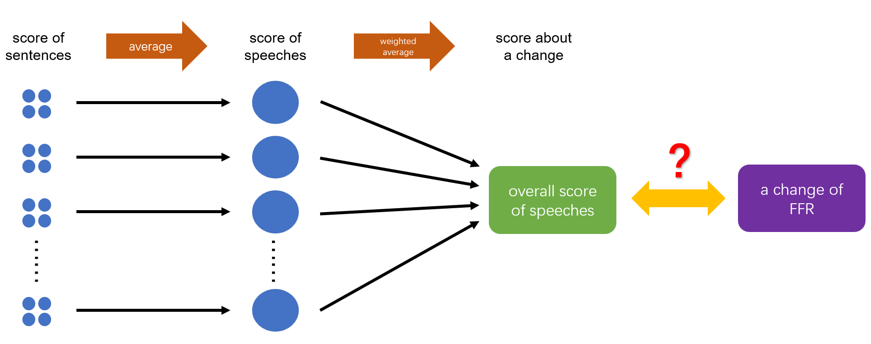
We used LM dictionary to calculate the polarity score of each sentence in a lecture and take the mean score of sentences in a speech as the overall sentiment of the lecture. Finally, we kept the score of each lecture in the dataframe and named it ’score_final‘.
import pysentiment as ps
#coding:utf8
lm = ps.LM()

score=[]
for i in range(len(df1['content'])):
    score_list=[]
    for j in range(len(df1['content'][i])):
            df1['content'][i][j]=cleaning_repeating_char(df1['content'][i][j])
            df1['content'][i][j]=cleaning_punctuations(df1['content'][i][j])
            score_of_one_sentence= lm.get_score(lm.tokenize(df1['content'][i][j]))['Polarity']
            score_list.append(score_of_one_sentence)
    score.append(np.mean(score_list))

Score=pd.DataFrame(score)
df=pd.concat([Score,df1],axis=1)

df=df.rename(columns={0:"score_final"})
Basis on Modeling
After analyzing the sentiment of the FOMC speeches and giving a sentiment score to each of them, we needed to build a connection between the score of speeches and the change in the federal funds rate (FFR). Actually, for each speech, there were two problems behind us: a) Which change of FFR does the speech have an influence on? b)There are 915 speeches in the dataset in total, but only 129 changes in FFR. Obviously, in most cases, a change is associated with more than one speech. So how to allocate the influence level (also known as weight) of different speeches to the same related change?
The federal fund's target rate is determined by a meeting of the members of the FOMC which normally occurs eight times a year.
And the interval between two adjacent meetings is about six to seven weeks. Since the decision of the change of FFR is made at the meetings and it exactly reflects the latest views of FOMC members on the recent economic situation and monetary policy, we believed only several latest speeches before a change imply the present views of the members and have a relationship with this change.
But what is the definition of ‘latest’? We thought only the speeches between the last meeting and this meeting would be taken into consideration when analyzing the change of FFR at a meeting. The information in the speeches before the last meeting has already shown in the last change. (P.S. The speeches exactly given on the same day with an FOMC meeting will be allocated to the next change of FFR.)
Among all the speeches that have influence on the same change in FFR, we believed that the closer the speech is to the meeting, the greater its impact on the change. Therefore, the days between the speech and the related meeting are also an important parameter.
How about our dependent variable, the change of FFR? Definitely, here are three kinds of results in a total of the FFR’s change after a general FOMC meeting: a) Increase. (We use ‘1’ to represent this case.) b) Decrease. (‘-1’ is used to represent this case.) c) Stay unchanged. (Actually, this is the most common result. And we use ‘0’ when it happens.) The transformation was already made in the dataset.
Below is the code that we used to determine the related time of the FOMC meeting and the number of days before the meeting of every observation.
FFR = pd.read_excel('FFR.xlsx', usecols = [0, 2])
Lecture = pd.read_excel('final_lecture.xlsx')

# Change the format of date from 'string' to 'datetime.datetime'
FFR['date'] = pd.to_datetime(FFR.date)
Lecture['date'] = pd.to_datetime(Lecture.date)

lec = Lecture[['date', 'score_final']].sort_values(by = 'date').reset_index(drop = True)

# To decide the time of change that each speech is related to
lec['next_change'] = ''
for i in range(len(lec)):
    for j in range(len(FFR)):
        if FFR.iloc[j]['date'] > lec.iloc[i]['date']:
            lec.loc[i, 'next_change'] = FFR.iloc[j]['date']
            break

# Calculate the difference of days between the speech and the related change of FFR
lec['day_delta'] = ''
for i in range(len(lec)):
lec.loc[i, 'day_delta'] = (lec.iloc[i]['next_change'] - lec.iloc[i]['date']).days
But what about our problem b)? If there are 10 speeches between two meetings, how to calculate their different influence on the next change of FFR?
We decided to get a weighted average of the sentiment scores of all speeches between two meetings to be the ‘overall score’ which is related to the next change of FFR, and take research on the correlation between the 'overall score' and the actual change. The weights will have an inverse relationship with the time interval between the speeches and the corresponding change.
During this process, we used the idea of exponential moving average to decide the exact value of the weights of each observation. In the pandas package of Python, there is a function called ewm which is responsible for this calculation, but its application scenarios are somewhat different from the problems we face, so we made some changes of its function and define our weighted average function to be:
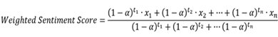
In this formula, x is the sentiment score of each speech, t is the days from the speech to the next FOMC meetings, and ‘alpha’ is a parameter to be determined. The larger the alpha, the greater the proportion of speeches that are close to the meetings in the overall score.
And here is the function we define in Python for this calculation:
def cal_avg(df, a):
    num = len(df)
    nume = 0
    deno = 0
    for i in range(num):
        score = df.iloc[i]['score_final']
        days = df.iloc[i]['day_delta']

        nume += (1-a)**days * score
        deno += (1-a)**days

return [nume/deno, num]
Since we couldn't decide the optimal value of alpha, we used traversal in the following process of model building.
Statistic Analysis
In general, the change of interest rates is a macroeconomic issue, and the traditional method of forecasting the decision of FOMC is to use factor models. (The factors, which are mainly economic indicators of the country, themselves are also an important basis for FOMC members to decide FFR.)
In this project, we firstly built a model based on the traditional way, using the economic factors to make predictions of changes of FFR. Then, we added the factor of sentiment scores about the speeches to the model, and saw if it could imporve the performance of the prediction model.
The macroeconomic indicators selected by us include:①Gross Domestic Product (GDP) ②Durable Goods Orders (DGORDER) ③Unemployment Rate (UNRATE) ④Procuder Price Index (PPIACO) ⑤Consumer Price Index less Food and Energy (CORESTICKM159SFRBATL)⑥Personal Consumption Expenditures (PCE) ⑦S&P 500 at close (S&P500_close)
In this part, we used yfinance and pandas_datareader to get the data of these economic indicators from trusted data sources.
import yfinance as yf
start = dt.datetime(2006, 1, 1)
end = dt.datetime.today()
sp = yf.Ticker('^GSPC')
sp_data = sp.history(interval = '1mo', start = start, end = end).reset_index()
sp_data = sp_data[['Date','Close']].rename(columns = {'Date':'DATE','Close': 'S&P500_close'})

import pandas_datareader as pdr
gdp_data = pdr.get_data_fred('GDP', start, end).reset_index()
dgo_data = pdr.get_data_fred('DGORDER', start, end).reset_index()
une_data = pdr.get_data_fred('UNRATE', start, end).reset_index()
ppi_data = pdr.get_data_fred('PPIACO', start, end).reset_index()
cpi_data = pdr.get_data_fred('CORESTICKM159SFRBATL', start, end).reset_index()
pce_data = pdr.get_data_fred('PCE', start, end).reset_index()
Then, we extracted the economic indicators which were corresponding to the timing of the FOMC meeting, and made them matched.
full_data = pd.DataFrame(meeting['date'])
full_data['year'] = full_data.date.apply(lambda x: x.year)
full_data['month'] = full_data.date.apply(lambda x: x.month)
full_data['quarter'] = full_data.date.dt.quarter

gdp_data['year'] = gdp_data.DATE.apply(lambda x: x.year)
gdp_data['quarter'] = gdp_data.DATE.dt.quarter
df = pd.merge(full_data, gdp_data, how = 'inner', on = ['year','quarter'])
full_data = pd.concat([full_data, df.GDP], axis = 1)

for data in [sp_data,dgo_data,une_data,ppi_data,cpi_data,pce_data]:
    data['year'] = data.DATE.apply(lambda x: x.year)
    data['month'] = data.DATE.apply(lambda x: x.month)
    df = pd.merge(full_data, data, how = 'inner', on = ['year','month'])
full_data = pd.concat([full_data, df.iloc[:,-1]], axis = 1)
After that, we defined a loop to traverse the alpha in the function of weighted average. The value range was from 0.01 to 0.5, per 0.01. When the alpha value was too large, the earlier speech had little effect on the change of FFR, which might not be a good model.
scores = pd.DataFrame(date,columns = ['date'])
for a in np.arange(0.01, 0.51, 0.01):
    summ = pd.DataFrame(columns = ['alpha_{}'.format(a)])
    for i in date:
        subdf = df[df['next_change'] == i]
        score, num = cal_avg(subdf, a)
        summ = summ.append({'alpha_{}'.format(a): score}, ignore_index = True)
scores = pd.concat([scores,summ],axis = 1)
We chose Random Forest as the classifier to build the model. First, we built a prediction model only using the macroecnomic indicators. Then, we added the factor of sentiment score to the model, and used different alphas to find out a model with the best performance.
from sklearn.ensemble import RandomForestClassifier
from sklearn.model_selection import train_test_split
yx = pd.merge(meeting, full_data, on = 'date')
yx = pd.merge(yx, scores, on = 'date').dropna()
y = yx.change
x_commen = yx.iloc[:,5:12]
RF = RandomForestClassifier(n_estimators = 200, max_depth = 3, random_state = 0)
X_train, X_test, y_train, y_test = train_test_split(x_commen, y, test_size = 0.33)
rf = RF.fit(X_train, y_train)
s_train = rf.score(X_train, y_train)
s_test = rf.score(X_test, y_test)

train_score = []
test_score = []
for x_score in yx.iloc[:,12:]:
    X_s = pd.concat([x_commen, yx[x_score]], axis = 1)
    Xs_train, Xs_test, y_train, y_test = train_test_split(X_s, y, test_size = 0.33)
    RF = RandomForestClassifier(n_estimators = 200, max_depth = 3, random_state = 0)
    rf_s = RF.fit(X_s, y)
    ss_train = rf_s.score(Xs_train, y_train)
    ss_test = rf_s.score(Xs_test, y_test)
    train_score.append((s_train, ss_train, ss_train - s_train))
test_score.append((s_test, ss_test, ss_test - s_test))
Using the above code, we built one model with traditional macroeconomic indicators, and 50 models containing the sentiment score of differnet alphas. We used the built-in function score calculating the mean accuracy of the model to evaluate the model performance.
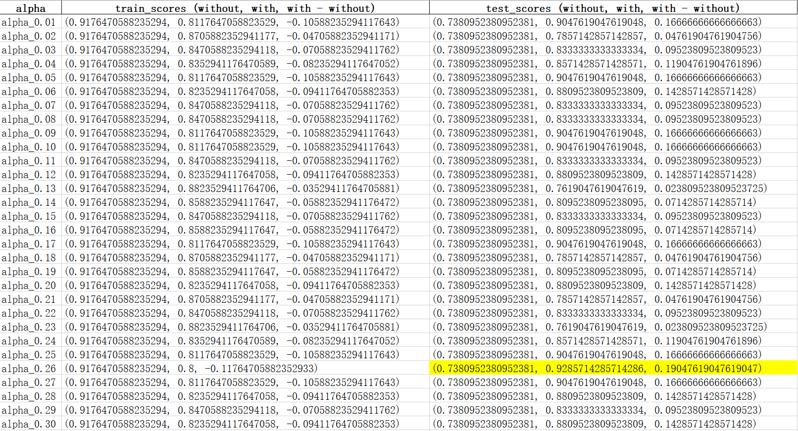
As could be seen from the figure, when applying the model to the training dataset, the model without the sentiment score outperforms the one with it. But as for the testing dataset, regardless of the value of alphas, the model with sentiment score has a better prediction power. Among all values of alpha, the model with sentiment score performs best when alpha is 0.26.
Conclusion
Compared with the result of the training dataset, the score of testing dataset is undoubtedly more convincing. Good performance in the training dataset may be due to overfitting, but a better performance in the testing dataset illustrates that the factor of sentiment score can significantly improve the generalization ability of the model. And in reality, what we are going to use the model to predict is a new sample that has never been seen before.
So we believe, the content of the FOMC speeches really helps when we make predictions about the next change of federal funds rate.