By Group "Citadel2"
Introduction
In this group project, we set out to analyse the effects of Fed speeches on cryptocurrency returns with natural language processing (NLP) techniques. Given this aim, it is all but necessary to 1) collect data in a timely and accurate manner, and 2) process and analyse the data such that we can generate actionable insight with economic value. In this blog, we aim to shed some light on our process, as well as some of the challenges we faced.
Data Collection
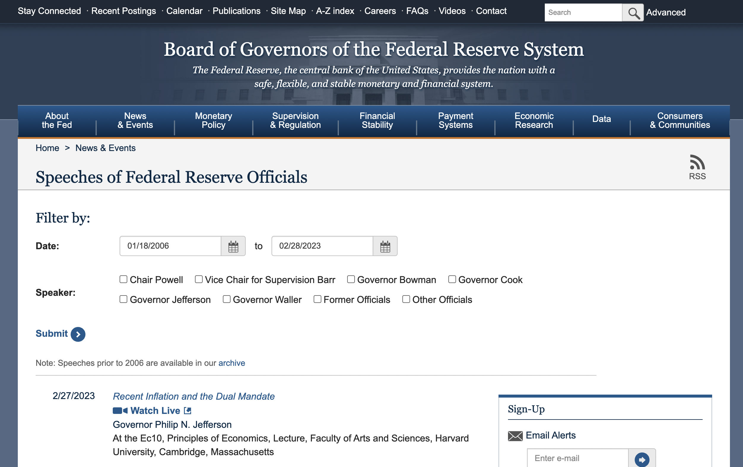
After each speech, their transcripts are uploaded to the Federal Reserve website.
This allows us to use the following script to scrape the website and download the speeches:

Then we define a function to scrape these speech texts, mainly using Chrome webdriver from Selenium. To scrape all speeches and store into one dataframe, we first get URLs of these speeches by using find_element function in Selenium from the whole page and then locate the "Next" button to turn to next page. We used newspaper3k to get speech content and BeautifulSoup to get article time.
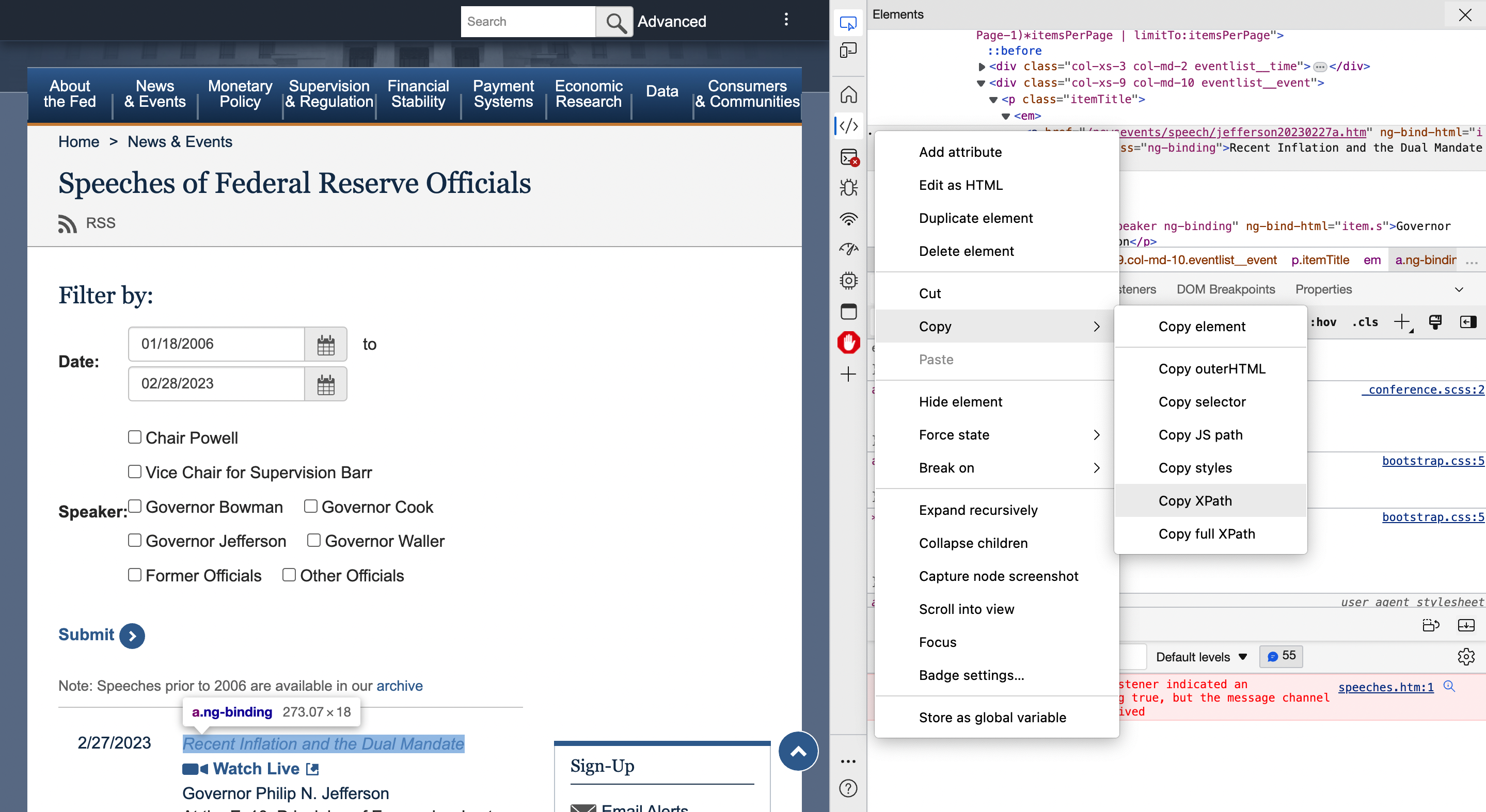
Here's an example using DEV tool to find the URL's XPATH:

The following is our scrape function:
def scrape_FR_speech():
    # scrape multiple FR speech text data
    driver = webdriver.Chrome()
    # Navigate to a webpage with pagination links
    driver.get("https://www.federalreserve.gov/newsevents/speeches.htm")
    url=[]
    FR_speech = pd.DataFrame()
    for page in range(1,24):
        if page == 24:
            passage_num = 13
        else:
            passage_num = 21

        for x in range(1,passage_num):
        XPath='//*[@id="article"]/div[1]/div['+str(x)+']/div[2]/p[1]/em/a'
            url= driver.find_element(By.XPATH, XPath).get_attribute('href')

            article = Article(url)
            article.download()
            article.parse()
            t = article.text
            df = pd.DataFrame([t], columns=['minutes'] )
            df['url'] = url

            # get article time
            response = requests.get(url)
            html_content = response.text

            # Parse the HTML content with BeautifulSoup
            soup = BeautifulSoup(html_content, 'html.parser')
            article_time = soup.find('p',class_='article__time').text
            article_time = datetime.datetime.strptime(article_time,"%B %d, %Y")
            df['article_time'] = article_time
            FR_speech= FR_speech.append(df)

        driver.find_element(By.LINK_TEXT,"Next").click()

    return FR_speech
Data Processing
For our purposes, speeches by Federal Reserve officials are a great source of text data, as they contain no gibberish, and the formal language allows for easy data augmentation – thus minimal cleaning is needed (compared to, for example, social media posts, which often contain abbreviations, emojis, slangs and/or colloquial language). However, we still need to inspect and clean the data – in case the downloaded text differs from that of the actual speech due to unexpected issues during web-scraping.
We first used the following code to drop references in the speech text:
# Drop reference in speech text
for count, item in enumerate(FR_speech['minutes']):
   lst = item.split('\n')
   item = ''.join(lst)

   # drop reference
   lst = item.split('Reference')
   item = lst[:1]
   item = "".join(item)

   # drop notes
   lst = item.split('. Return to text')
   item = lst[:1]
   item = "".join(item)

   FR_speech['minutes_cleaned'][count] = item
We then removed useless characters, and converted all letters to lowercase:
def pre_process(text):

    # Remove links
    text = re.sub('http://\S+|https://\S+', '', text)
    text = re.sub('http[s]?://\S+', '', text)
    text = re.sub(r"http\S+", "", text)
   # remove the reference numbers
    text = re.sub(r'.\d+', '.', text)
   # Remove multiple space characters
    text = re.sub('\s+',' ', text)
   # Convert to lowercase
    text = text.lower()
   return text
Now we can summarize the article, by removing stop words, then calculating the relative frequencies of each word, and finally rank each sentence by its relative importance:
# Summarized the article (remove insignificant sentences)

def sum_article(text):
    from spacy.lang.en.stop_words import STOP_WORDS
    from sklearn.feature_extraction.text import CountVectorizer
    import en_core_web_sm
    nlp = en_core_web_sm.load()
    doc = nlp(text)

   # remove create a dictionary of words and their respective frequencies
    corpus = [sent.text.lower() for sent in doc.sents ]
    cv = CountVectorizer(stop_words=list(STOP_WORDS))
    cv_fit=cv.fit_transform(corpus)
    word_list = cv.get_feature_names();
    count_list = cv_fit.toarray().sum(axis=0)
    word_frequency = dict(zip(word_list,count_list))

    # compute the relative frequency of each word
    val=sorted(word_frequency.values())
    higher_word_frequencies = [word for word,freq in word_frequency.items() if freq in val[-3:]]

    # gets relative frequency of words
    higher_frequency = val[-1]
    for word in word_frequency.keys():
        word_frequency[word] = (word_frequency[word]/higher_frequency)

    # Creating a ordered list (ascending order) of most important sentences
    sentence_rank={}
    for sent in doc.sents:
        for word in sent :
            if word.text.lower() in word_frequency.keys():
                if sent in sentence_rank.keys():
                    sentence_rank[sent]+=word_frequency[word.text.lower()]
                else:
                    sentence_rank[sent]=word_frequency[word.text.lower()]
    top_sentences=(sorted(sentence_rank.values())[::-1])
    top_sent=top_sentences[:10]

    summary=[]

    for sent,strength in sentence_rank.items():
        # print(sent)
        if strength in top_sent:
            # summary.append(sent)
            temp = ''.join(str(sent))
            summary.append(temp)
        else:
            continue
    return ' '.join(summary)
Next, we split the passage into sentences using the NLTK sentence tokenizer, then finally removing outliers and errors before putting the data through the natural language processing model.
# Turn passage to sentences
tokenizer = nltk.data.load('tokenizers/punkt/english.pickle')
FR_speech['Sentences'] = FR_speech['summarized_article'].apply(tokenizer.tokenize)

# Explode sentences into separate rows, keeping other data
FR_speech = FR_speech.explode('Sentences').reset_index(drop=True)

# Drop the outliers

FR_speech['Sentences_length'] = pd.Series()
for count, item in enumerate(FR_speech['Sentences']):
    FR_speech['Sentences_length'][count] = len(item)
FR_speech['Sentences_c'] = FR_speech[ FR_speech['Sentences_length']>= len ]['Sentences']
FR_speech = FR_speech.dropna()
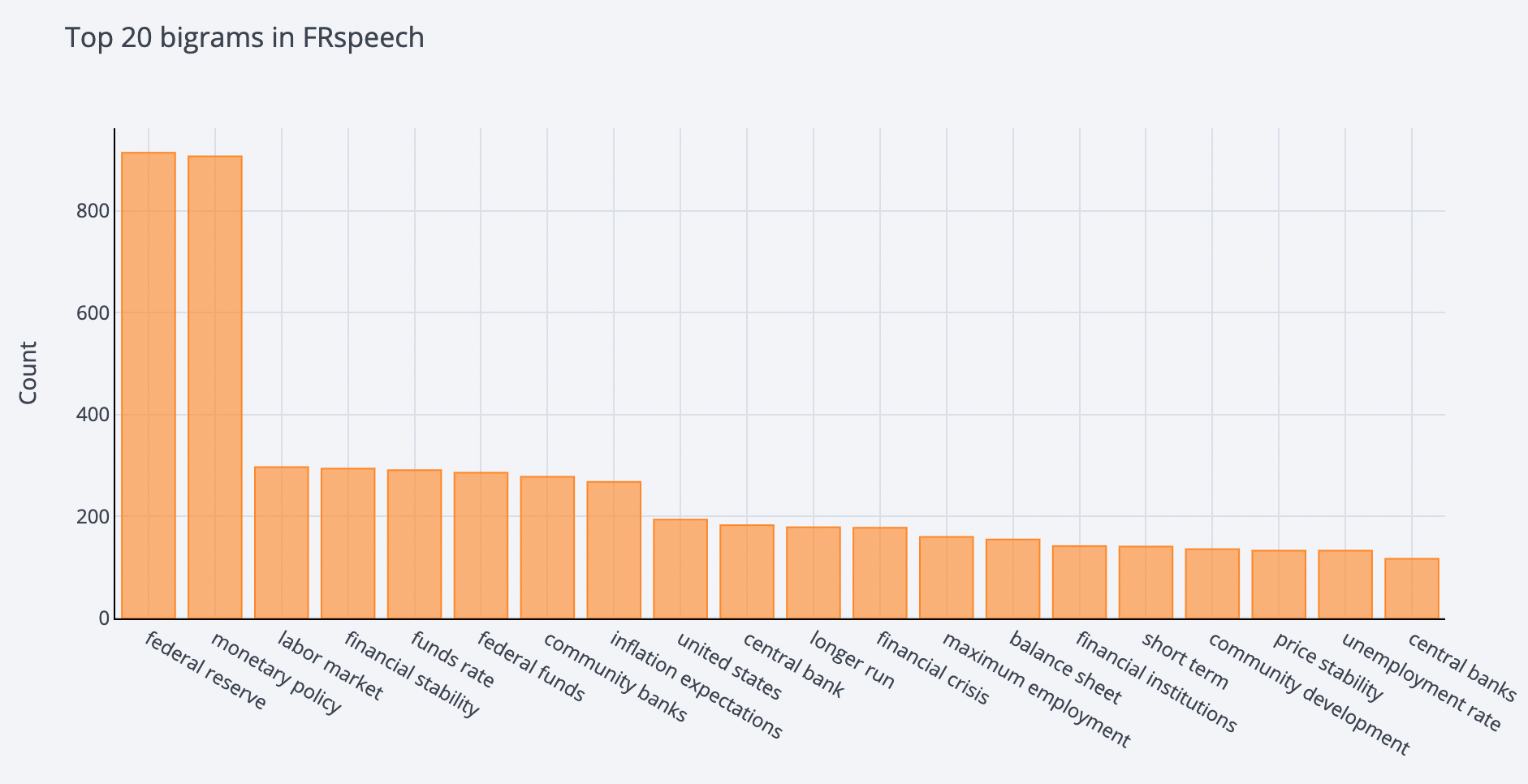
Here's top 20 bigrams from cleaned speech text:

Model Evaluation
For the model evaluation part, our initial idea was to directly link sentiment to price direction, but it would not be precise enough since other factors could affect it, so a two-model approach was selected in our project. The first step is to establish a model to determine the sentiment score, then use sentiment score and other factors to determine bitcoin price fluctuations. We changed our approach several times for the first model.
We first considered supervised machine learning with manually labelled data, but it is costly and time-consuming. Then, we regarded VADER as our second choice since VADER is a relatively simple and straightforward method with a lower computation cost. Additionally, unlike machine learning which requires the same format of the input, it does not require a fixed sentence length. Accordingly, we did a test to determine whether this method is appropriate or not. We imported a training set with an assumed 100% accuracy, then we converted positive sentiments to 1, negative to -1, and 0 otherwise.
def clean_sentiment(text):
    if text == 'positive' or text == 'pos':
        return 1
    elif text == 'negative' or text == 'neg':
        return -1
    else:
        return 0
After that, we used the VADER code to generate sentiments from the text.
def VADER_polarize_by_max(text):
    scores = sid.polarity_scores(text)
    scores.pop('compound', None)
    label = max(scores, key=lambda k: scores[k])
    return clean_sentiment(label)

def VADER_polarize_by_compound(text):
    score = sid.polarity_scores(text)['compound']
    if score > 0:
        return 1
    elif score < 0:
        return -1
    else:
        return 0

def TextBlob_polarize_by_compound(text):
    score = TextBlob(text).sentiment.polarity
    if score > 0:
        return 1
    elif score < 0:
        return -1
    else:
        return 0
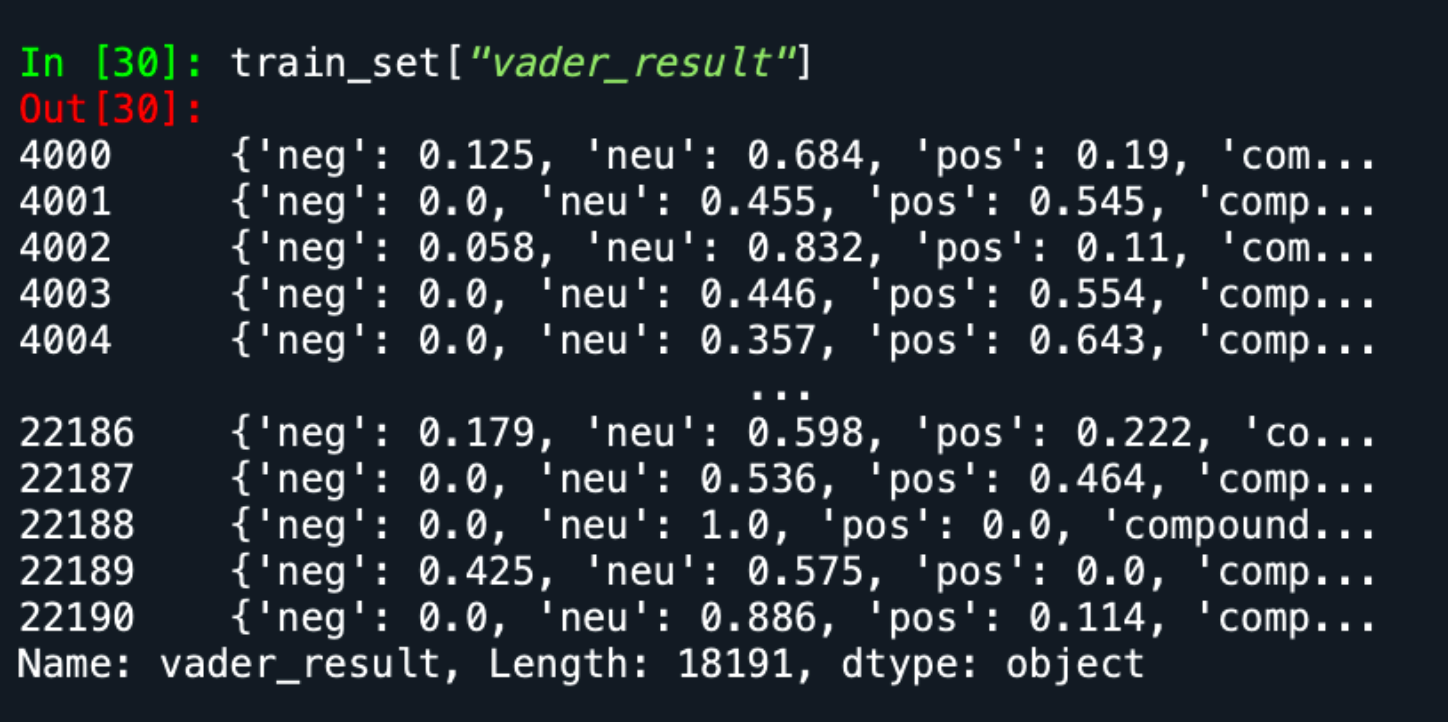
Here's the result using VADER:

Unfortunately, the accuracy rate was only 53%, which is too low.
In this case, we believe that the low accuracy rate can be explained by the nature of the VADER model. VADER is a rule-based sentiment analysis model without explicitly coding it. For example, the score would be '+1' if the sentence has hawkish keywords and more positive than negative terms, and '-1' if the sentence conveys a dovish sentiment. This method can also be described as lexicon-based, where a sentiment score heavily relies on the polarity and intensity of the sentiment of a single word. All of this means that the VADER model ignores the contextual information as the BoW and TF-IDF.
We also considered unsupervised machine learning. However, its input data is not labelled by people in advance, instead the testing data is grouped automatically. Although no training set is required for unsupervised machine learning, the automated grouping may not be desirable as there is no particular indication. With a large number of specialised words in Federal Reserve speeches, it is impossible to tell the computer how to distinguish between these sentiments.
Therefore, after taking into account the pros and cons of each method, we decided to use supervised machine learning with different training sets (FiQA and FinancialPhraseBank). While this method has one limitation - in that these training sets are not entirely based on bitcoin, we can improve the accuracy by tuning and refining some parameters by ourselves, such as dropout, leaning rate, and weight decay.
Next Steps
After collecting and processing the Fed speech text data and the Bitcoin price data, as well as evaluating different methods for sentiment analysis, our next steps would be to put everything together and find insights on how Fed speeches factor into cryptocurrency returns. See more details in our next blog.