By Group "Citadel2"
Introduction
After having obtained and processed the raw data, we now need to set up the models required for analysing the speeches and price data. To do so, model training with cleaned training data is necessary. Let's take a look at our process below.
Data Cleaning of Training Set
First, we define a couple of functions to clean the training set, FiQA and Financialphrase bank.
The original data looks like:
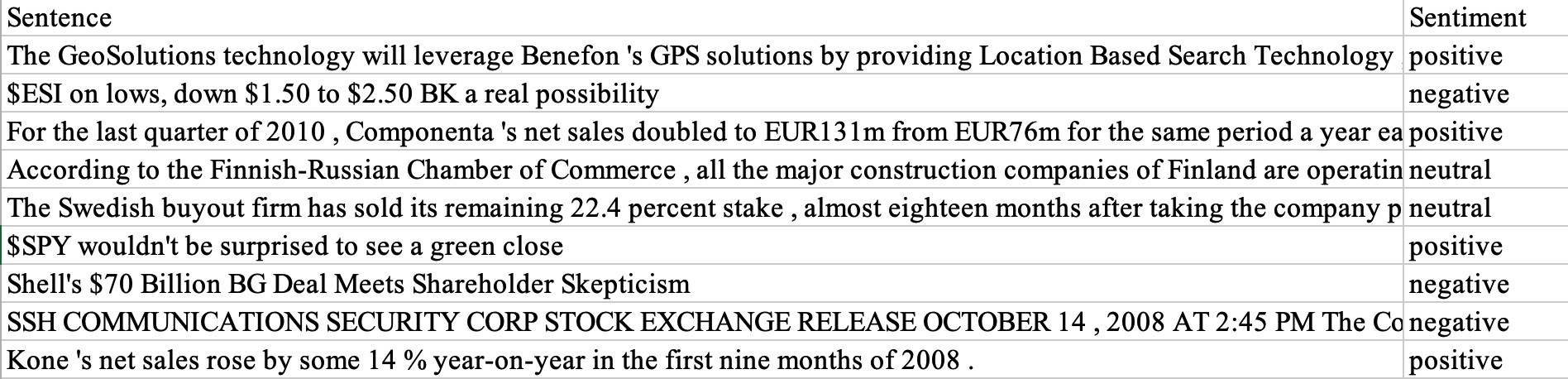
We convert words (‘positive’, ‘negative’, ‘neutral’) into numbers (1, -1, 0), and then convert numbers into vectors ([1, 0, 0], [0, 0, 1], [0, 1, 0]). By using the word-vector representations, we directly apply suitable machine learning algorithms to solve the problems that we have at hand, like sentiment analysis.
def clean_sentiment(text):
    if text == 'positive' or text == 'pos':
        return 1
    elif text == 'negative' or text == 'neg':
        return -1
    else:
        return 0

def soft(text):
    if text == 1:
        return [1, 0, 0]
    elif text == -1:
        return [0, 0, 1]
    else:
        return [0, 1, 0]
There is a lot of useless information containing features that result in noise for sentiment analysis, such as hyperlinks, new line characters, mentions, hashtags and more, so we also remove them.
def pre_process(text):
text = str(text)
# Remove links
text = re.sub('http://\S+|https://\S+', '', text)
text = re.sub('http[s]?://\S+', '', text)
text = re.sub(r"http\S+", "", text)
# Convert HTML references
text = re.sub('&', 'and', text)
text = re.sub('<', '<', text)
text = re.sub('>', '>', text)
text = re.sub('\xa0', ' ', text)
# Remove new line characters
text = re.sub('[\r\n]+', ' ', text)
# Remove mentions
text = re.sub(r'@\w+', '', text)
# Remove hashtags
text = re.sub(r'#\w+', '', text)
# Remove multiple space characters
text = re.sub('\s+', ' ', text)
pattern = re.compile(r'\b(' + r'|'.join(STOPWORDS) + r')\b\s*')
text = pattern.sub('', text)
text = text.lower()
return text
Besides, the contractions package can restore common English abbreviations and slangs, and is efficient in handling edge cases, such as missing apostrophes. Therefore, we use contractions to reduce dimensionality and further filter stopwords.
def expand_contractions(text):
    try:
        return contractions.fix(text)
    except:
        return text
Next, we split up the text into smaller parts by using the function get_tokenizer() and convert 1D to 2D.
Finally, we load the word vectors and call all the defined functions.
tokenizer = get_tokenizer('basic_english')
def text_transform(sentence, maxSeqLength):
    sentence_vector = []
    for token in tokenizer(sentence):
        try:
            sentence_vector.append(wordsList[token])
        except:  # exclude non english sentence and not recognized word (gibberish)
            sentence_vector.append(0)
    if len(sentence_vector) > maxSeqLength:
        sentence_vector = sentence_vector[:maxSeqLength]
    elif len(sentence_vector) < maxSeqLength:
        sentence_vector.extend(np.zeros(maxSeqLength - len(sentence_vector), dtype='int64'))
    return sentence_vector
RNN model
In our example, we split 80% of the training set for training and the other 20% of the data is used for validation.
Now that we have the processed, cleaned text, we apply pretrained embeddings in conjunction with the RNN model for sentiment analysis to obtain the subjectivity and polarity of sentences.
Compared with self-training embeddings, pretrained embeddings can reduce the number of parameters to train, hence reducing the training time. Since pretrained embeddings have previously been trained on a vast corpus of text, they can capture both the connotative and grammatical meanings of a word, as well as reduce overfitting of the RNN model. nn.Embeddings is then used to create a 2d matrix. By using RNN, we encode the similarity and dissimilarity between words, and can access vector elements by index. We also use max_seq_length, which specifies the maximum number of tokens of the input.
In the following RNN class, while each token of a text sequence gets its individual pretrained representation via the embedding layer (self.embedding), the entire sequence is encoded by a RNN (self.rnn). More concretely, the hidden states (at the last layer) of the RNN at both the initial and final time steps are concatenated as the representation of the text sequence.
We also adopted layer normalization, which applies per-element scale and bias with elementwise_affine, to enable smoother gradients and faster training.
class RNN(nn.Module):
    #   pretrained embedding
    def __init__(self, wordVectors, embedding_dim, hidden_dim, num_layers, output_dim, maxseqlength):
        super().__init__()
        self.embedding = nn.Embedding.from_pretrained(torch.from_numpy(wordVectors).float())
        self.rnn = nn.RNN(embedding_dim, hidden_dim, num_layers=num_layers)  # similar to one hidden layer
        self.fc = nn.Linear(maxseqlength * hidden_dim, output_dim)
        self.hidden_dim = hidden_dim
        self.maxseqlength = maxseqlength
        self.ln = nn.LayerNorm([maxseqlength, embedding_dim], eps=1e-05, elementwise_affine=True)
Let’s construct a RNN by using Kaiming Initialization, which considers the non-linearity of activation functions, to represent single text for sentiment analysis. The fully connected layer is used to calculate the sentiment stored in the hidden layer and to sum up the sentiment of the entire sentence.
        def _weights_init(m):
            """ kaiming init (https://arxiv.org/abs/1502.01852v1)"""
            if isinstance(m, nn.Linear) or isinstance(m, nn.Conv2d):
                nn.init.kaiming_normal_(m.weight)
            elif isinstance(m, nn.BatchNorm2d):
                nn.init.constant_(m.weight, 1)
                nn.init.constant_(m.bias, 0)
        self.apply(_weights_init)

    def forward(self, x): # text = [batch size, sent len]
        embedded = self.embedding(x) # embedded = [batch size, sent len, emb dim]
        embedded = self.ln(embedded)
        out, hidden = self.rnn(embedded) # output = [batch size, sent len, hid dim] # hidden = [1, sent len, hid dim]
        out = out.view(out.size(0), self.maxseqlength * self.hidden_dim)
        out = self.fc(out) # output = [batch size, output size]
        return out
Now we can summarize the article, by removing stop words, then calculating the relative frequencies of each word, and finally rank each sentence by its relative importance.
Training Process
We define the train_model() function for training and evaluating the model.
def train_model(model, args):

    checkpoint_dir = args.checkpoint_dir
    if not os.path.exists(checkpoint_dir):
        os.makedirs(checkpoint_dir)

    optimizer = torch.optim.AdamW(model.parameters(), betas=(0.9, 0.999), weight_decay=args.weight_decay,
                                  lr=args.learning_rate)
    scheduler = torch.optim.lr_scheduler.LambdaLR(optimizer, lambda epoch: 0.99 ** epoch)
    criterion = nn.CrossEntropyLoss() #  nn.BCELoss(reduction='mean')
We need to pass the entire dataset multiple times through the same RNN as we are using a limited dataset and gradient descent, which is an iterative process. Therefore, we start by looping through the number of epochs, and the number of iterations in each epoch is set according to the batch size that we defined. We pass the text to the model and get the predictions from it. In this way, sentences are assigned scores for positive, neutral and negative sentiments. Finally, we calculate the loss for each iteration (the discrepancy between the true and our predicted sentiment) to get the average loss.
    # load optimizer and epoch
    start_epoch = 0
    if args.load_pretrain:
        checkpoint = torch.load(os.path.join(checkpoint_dir, 'model_epoch_' + str(args.which_checkpoint) + '.pth'))
        optimizer.load_state_dict(checkpoint['optimizer'])
        scheduler.load_state_dict(checkpoint['scheduler'])
        start_epoch = checkpoint['epoch']

    for epoch in range(start_epoch, args.num_epochs):
        model.train()
        total_loss = 0.
        progress_bar = tqdm.tqdm(enumerate(train_loader), total=len(train_loader))

        for i, (x, y) in progress_bar:
            y_pred = model(x)
            loss = criterion(y_pred.float(), y.float())  # float prevent tensor type difference
            total_loss += loss.data

            optimizer.zero_grad()
            loss.backward()
            optimizer.step()

            avg_loss = total_loss / (i + 1)
            if (i + 1) % 5 == 0:  # every 5 batch
                print('Epoch [%d/%d], Iter [%d/%d] Loss: %.4f, average_loss: %.4f' % (epoch + 1,
        args.num_epochs, i + 1, len(train_loader),loss.data, avg_loss))
        if args.scheduler == True:
            scheduler.step()

        model.eval()
Next, we want to validate our model performance during training by using the validation set. We then save the sentiment analysis model that has the best validation loss and the best accuracy, as well as each loop and loss.
Prediction Process
Since the model is created and data is trained and evaluated, we make a prediction by using predict() function, which is more efficient when it comes to large arrays of data.
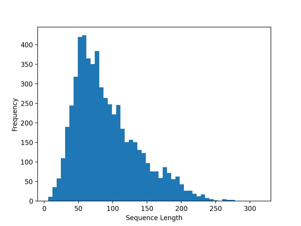
senquence_length is an important variable to set, we first draw a histogram to decide which number to choose:
Then we use the following predict function to gain sentiment scores:
def predict(args, model):
    test_path = args.test_path
    df = pd.read_parquet(test_path)
    df = pd.DataFrame(df)
    df.rename(columns={'Sentences_c':'sentence'}, inplace=True)
    df['sentence'] = df['sentence'].apply(expand_contractions)
    raw_sentence = df['sentence']
    df['sentence'] = df['sentence'].apply(lambda sentence: text_transform(sentence,\
             maxSeqLength=args.maxSeqLength))
    df = df.dropna()

    print('PREDICTING...')

    pred_list = []
    for idx in range(df.shape[0]):
        with torch.no_grad():
            x = df['sentence'].iloc[idx]
            x = torch.tensor(x).unsqueeze(0) # same as batch input (batch_size, sequence_length)
            y_pred = model(x) # 2d tensor
            y_pred = nn.functional.softmax(y_pred, dim=1)
            y_pred = torch.flatten(y_pred) # 1d tensor
            pred_list.append(y_pred.tolist()) # pred_list: 2d list

    pred_matrix = np.matrix(pred_list) # pred_matrix [samples, 3] 3: [posive, neutral, negative]
    df['positive sentiment'] = pred_matrix[:, 0]
    df['negative sentiment'] = pred_matrix[:, 2]
    df['sentence'] = raw_sentence
    df.to_csv(os.path.join(result_dir, 'sentiment_result.csv'))
To achieve this goal, we first create an ArgumentParser() object, then call the add_argument() method to add parameters, which have all been defined in the training process. And lastly, we use parse_args() to parse the added arguments.
if __name__ == '__main__':
    parser = argparse.ArgumentParser()
    # model settings
    parser.add_argument('--EMBEDDING_DIM', default=50, type=int)  # wordVectors.shape[1] = 50
    parser.add_argument('--HIDDEN_DIM', default=128, type=int)
    parser.add_argument('--OUTPUT_DIM', default=3, type=int)  # -1, 0, 1
    parser.add_argument('--NUM_LAYERS', default=2, type=int)
    parser.add_argument('--maxSeqLength', default=81, type=int) # from the train_sentiment.py: np.median(sequence_length)
    # files path
    parser.add_argument('--test_path', default='project/dataset/test/sentiment.parquet',
                        type=str)
    parser.add_argument('--checkpoint_dir', default='project/checkpoints', type=str,
                        help='output directory')
    parser.add_argument('--lexicon_dir', default='project', type=str)
    parser.add_argument('--result_dir', default='project/result', type=str)

    args = parser.parse_args()
Next, we instantiate RNN model with relevant parameters and finally get to test our model to see what kind of output we will get.
    result_dir = args.result_dir
    if not os.path.exists(result_dir):
        os.makedirs(result_dir)

    model = RNN(wordVectors=wordVectors, embedding_dim=args.EMBEDDING_DIM,hidden_dim=args.HIDDEN_DIM,
            num_layers=args.NUM_LAYERS, output_dim=args.OUTPUT_DIM,\
        maxseqlength=args.maxSeqLength)

    print('LOADING MODEL...')
    model.load_state_dict(torch.load(os.path.join(args.checkpoint_dir, 'model_best.pth'))['model'])
    model.eval()

    predict(args, model)
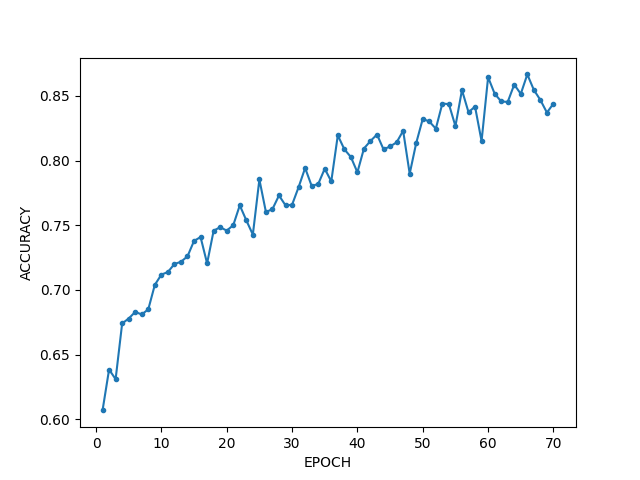
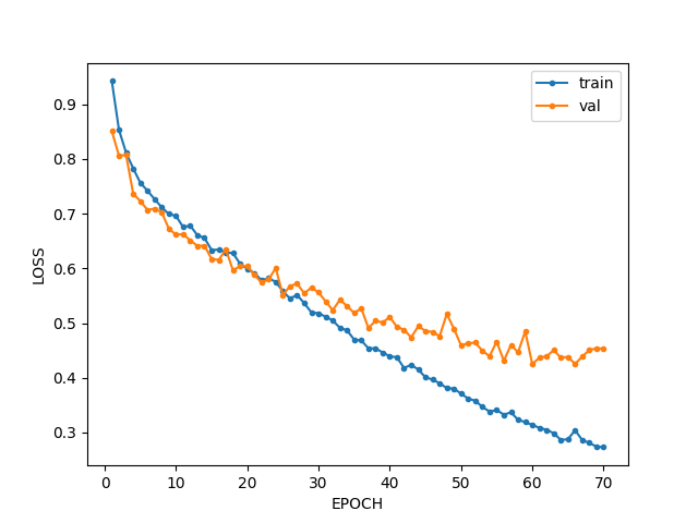
Luckily, the results returned are encouraging and we plot them as follows:
Next Steps
Now that we have the tools for analysing the speeches, we can use the results to generate actionable insights for trading cryptocurrencies.