By Group "PoliVoli"
X Selection
Currently, there are two approaches within the team regarding the selection of the X variable. The first involves using the outputs from three distinct sentiment models as the variable. The second approach does not rely on other sentiment models; instead, it exclusively employs the tokenization tool provided by ProsusAI within Finbert to vectorize Trump's speech for independent training.
Corresponding to each different X variable, we conducted separate model training sessions.
Y Selection
In the previous blog, we proposed three methods for constructing Y: labeling daily volatility using the population sample mean or median; assessing the persistent effect of X using delta+n; and determining the short-term effect by subtracting the day's low from its high. Given the interpretability of the framework and regression results, direct labeling via mean or median proved infeasible. However, the combined approach using methods two and three—estimated by ‘h-l day+1’ (the next day's high-low range)—demonstrated both economic and statistical significance. 'large vol' is calculated based on ‘h-l day+1’ to determine whether this value ranks within the top 25% (75th percentile) over the past 40 days. Using 20% would result in insufficient data meeting the subsequent overlay requirements. The 25% threshold represents one-quarter, aligning with standard practice. Verification confirmed all desired dates (e.g., April 7th tariffs) meet this criterion. The final calculated variable ‘y’ is ‘pos large’, signifying a positive large volatility event. Its underlying logic is: if (‘delta+1’ > 0), then ‘delta+1’; otherwise, 0. This means if the large volatility is a sharp decline in VIX, it would be 0. Only a significant upward volatility on the following day would yield a value of 1. ‘delta+1’ is calculated as the next day's closing price divided by today's closing price minus 1. The reason for distinguishing positive and negative values is our assumption that Trump's speeches will increase volatility. However, if we only judged amplitude (high-low), a significant drop in volatility would also yield a value of 1, contradicting our original intent. Therefore, we need to add a layer of directional judgment.
The primary code as follows:
import pandas as pd import numpy as np
from datetime import datetime, timedelta

df['(high-low)/today_price'] = (
    df['recent_40_days_75%_percentile']
      .rolling(window=40, min_periods=40)
      .quantile(0.75)
      .shift(-39)
)
df['whether_big_vol'] = (
    (df['(high-low)/today_value'] >= df['recent_40days_75%_percentile'])
    .astype(float)
    &
    (df['(high-low)/today_value'] > df['(high-low)/today_value'].shift(1))
    .astype(float)
)
Random Forest Tree Model
Feature Construction (X Selection)
Yang et al. (2020) show that FinBERT performs well in financial tasks such as sentiment analysis and event extraction, and that its embeddings preserve financial semantics, making them suitable for time-series financial data. So, in our project, we use the FinBERT model to train the text data to gain the daily superimposed vectors of Trump and use them to find the relation between volatility and these vectors. We use the FinBERT code gained from ProsusAI in Hugging Face (2021) to train the FinBERT model. Firstly, we attempt sentiment analysis of single-date text in 2025-10-10 and this model extracts the text list for the date, and then it performs text encoding via tokenizer to get the logits and transfer the probability of positive, negative or neutral by using the softmax. Finally, it match the built-in label mapping of the model dynamically which aims at avoiding hard coding, and output the three probabilities of each text and the final predicted emotion label. These codes are displayed by 1.py document. After training, we download the result of the vectors in 2.py shown in picture 1 and I find that the FinBERT model adopts 768-dimension vector which is too large for this project because our data volume only is about 2000, so we reduce the dimension of this vector to 128-dimension by pca (Hasan and Abdulazeez,2021).

Y Selection
Additionally, Trump always posts several posts each day and we only have the daily volatility data so we should sum these vectors from text data in the same day to match the date of volatility shown by 7.py. Meanwhile, we merge the 128-dimension vector of text data and volatility data to prepare for machine learning. However, in this step, we original select the the difference of the volatility in two consecutive trading days as the dependent variable, and we assume the dependent variable y as the difference of volatility in two consecutive trading days exceed positive and negative 0.9 standard deviation (using the sd of the closest 40 trading days ) as the label 1, then we can use random forest to train the module, but in fact, we should attempt to adjust the value of sd to gain a suitable result based on the result of machine learning because there is no standard to show what range of fluctuation is considered abnormal, which means y could exceed positive or negative 0.5, 0.9 or other number and 128-dimension vector may also be large so we use for-loop to run the results based up on different values of dimension. Thus, there problem should be addressed while using random forest model.
Model Training
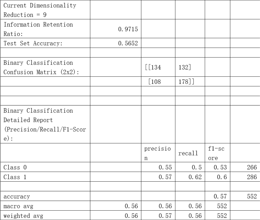
Random forest is a good model to address the overfitting problem so it could be used in the classification problem because it is suitable for high-dimension data with high robustness (Breiman,2001). We randomly select the train dataset and test dataset with ratio 7:3, and the independent variables are the 128-dimension vectors in each trading day and the dependent variable y defined before. And we define that the type 0 is the volatility of the second day is in range of the first day minus and add the sd with relevant coefficient, and the remaining are of type 1. To maximize the precision, we select n_estimator with 800 and shows the precision when reducing the dimensions of the vector from 3 to 64. We find that there is almost no difference when the dimension is above 21. Therefore, we only display the results with the dimension between 3 to 21. Afterwards, we adjust different numbers of the sd to run random forest model. Meanwhile, in order to use the precision and recall to measure the reliability of the model, the confusion matrix is used. Finally, we find that the best result shown in picture2 (11.py document) is when the dimension is 9 and y should exceed positive or negative 0.514 sd. We find that the recall and precision of type 0 and 1 are both higher than 50%, which shows that Trump’s posts have relationship with volatility in some degree. However, this result does not mean the next step that is our strategy will use the result since it depends on the profit gained based on the model. Therefore, we keep many types of labels with 21 different numbers of the coefficient to use further.
XGBoost Tree Model
Feature Construction (X Variables)
In the XGBoost model, we constructed independent variables from a textual sentiment perspective, primarily employing three sentiment analysis methods: TextBlob, VADER, and FinBERT. Additionally, we introduced a feature based on text length.
First, we used the TextBlob module to extract two continuous sentiment variables: Polarity and Subjectivity. Subsequently, the VADER sentiment analyzer calculates four sentiment scores: vader_neg, vader_neu, vader_pos, and vader_compound. Thus, TextBlob and VADER collectively provide six dictionary- and rule-based sentiment variables.
The primary code for the TextBlob and VADER modules is as follows:
from textblob import TextBlob
import nltk
nltk.download('punkt_tab')
nltk.download('averaged_perceptron_tagger')
for i in range(len(df)):
    text = df.iloc[i, 3]
    if pd.isnull(text):
        polarity_list.append(None)
        subjectivity_list.append(None)
    else:
        blob_par = TextBlob(text)
        polarity_list.append(blob_par.sentiment.polarity)
        subjectivity_list.append(blob_par.sentiment.subjectivity)

df['Polarity'] = polarity_list
df['Subjectivity'] = subjectivity_list

import re
from nltk.sentiment.vader import SentimentIntensityAnalyzer
analyzer = SentimentIntensityAnalyzer()
for i in range(len(df)):
    text = df.iloc[i, 3]
    if pd.isnull(text):
        vader_neg.append(None)
        vader_neu.append(None)
        vader_pos.append(None)
        vader_compound.append(None)
    else:
        score = analyzer.polarity_scores(text)
        vader_neg.append(score['neg'])
        vader_neu.append(score['neu'])
        vader_pos.append(score['pos'])
        vader_compound.append(score['compound'])
Second, we introduce the pre-trained FinBERT model to predict sentiment classification probabilities for tweet texts, yielding probability outputs for three sentiment categories: positive (p_pos), negative (p_neg), and neutral (p_neu).
The main code body is as follows:
import torch
import numpy as np
import pandas as pd
from transformers import AutoTokenizer, AutoModelForSequenceClassification
from tqdm.auto import tqdm

model_name = "ProsusAI/finbert"
tokenizer = AutoTokenizer.from_pretrained(model_name)
model = AutoModelForSequenceClassification.from_pretrained(
    model_name,
    use_safetensors=True
)
model.eval()

def finbert_score_df(
    df: pd.DataFrame,
    text_col: str = "content",
    batch_size: int = 32,
    max_length: int = 128
) -> pd.DataFrame:

    texts = df[text_col].astype(str).str.strip()
    mask = texts.ne("")
    idxs = df.index[mask]
    texts = texts[mask].tolist()

    probs_all = []

    for i in tqdm(range(0, len(texts), batch_size)):
        enc = tokenizer(
            texts[i:i + batch_size],
            return_tensors="pt",
            padding=True,
            truncation=True,
            max_length=max_length
        )
        with torch.no_grad():
            probs = torch.softmax(model(**enc).logits, dim=1).cpu().numpy()
        probs_all.append(probs)

    probs_all = np.vstack(probs_all)

    df[["p_pos", "p_neg", "p_neu"]] = np.nan
    df.loc[idxs, ["p_pos", "p_neg", "p_neu"]] = probs_all[:, [pos_id, neg_id, neu_id]]

    df["sent_dir"] = df["p_pos"] - df["p_neg"]
    df["sent_abs"] = (df["sent_dir"]).abs()

    return df

def count_words(text):
    if pd.isnull(text):
        return 0
    text = re.sub(r"[^A-Za-z0-9']", " ", text)
    words = text.split()
    return len(words)
df['word_count'] = df['content'].apply(count_words)
Based on this, we further construct two derived metrics:
sent_dir (Sentiment Direction Indicator): Composed of the difference between positive sentiment probability and negative sentiment probability, p_pos−p_neg, used to characterize the overall directionality of text sentiment;
sent_abs (Sentiment Intensity Indicator): The absolute value of the sentiment direction indicator, used to measure the degree to which text sentiment deviates from a neutral state.
Here, sent_dir emphasizes the positive or negative orientation of sentiment, while sent_abs captures the intensity of emotional expression. We believe directional and intensity-based sentiment features may carry distinct predictive implications in financial contexts, hence incorporating both into the model.In summary, the final X variable comprises 12 dimensions: 6 from TextBlob and VADER, 5 from FinBERT (3 raw probability variables plus 2 derived variables sent_dir and sent_abs), and 1 text length variable word_count. These features will be uniformly input into the XGBoost model for training and evaluation in subsequent steps.
Feature Integration
During the modeling process, directly mapping multiple text features (X) from the same trading day to the same daily market outcome variable (Y) for training inevitably introduces structural bias. The root cause lies in the fact that multiple texts released within a single trading day often pertain to different events or themes, thereby reflecting divergent or even conflicting sentiment information. However, during the data construction phase, these texts are uniformly mapped to the same market volatility label. This issue significantly increases intra-sample heterogeneity, making it difficult for the model to identify which sentiment features truly hold explanatory or predictive value. Consequently, it weakens the model's stability and generalization capabilities, potentially introducing systematic estimation bias during training.
Therefore, in subsequent modeling, we perform daily aggregation on text features from the same trading day. Specifically, for each sentiment variable corresponding to individual texts within the same day, we employ the mean as the primary aggregation method to characterize the overall sentiment level for that day.
For the Subjectivity variable from TextBlob, aggregation is performed using the sum method. This approach aims to capture the cumulative degree of subjective expression within the day's texts—that is, the overall intensity of sentiment expression on the subjective dimension for the day, rather than the average level of individual texts. Since subjectivity reflects the prominence of emotional or stance expressions in the text, its cumulative effect is more likely to influence the market's overall reaction to that day's information. Therefore, we employ summation for integration on this dimension.
df = (
    df1
    .groupby("trade_date", as_index=False)
    .agg({
        'p_pos': 'mean',
        'p_neg': 'mean',
        'p_neu': 'mean',
        'Polarity': 'mean',
        'Subjectivity': 'sum',
        'VADER_compound': 'mean',
        'sent_dir': 'mean',
        'sent_abs': 'mean',
        'word_count': 'mean',
        'VADER_neg': 'mean',
        'VADER_neu': 'mean',
        'VADER_pos': 'mean',
        'vol': 'max'
    })
)
Model Training
During the model training phase, we first perform a train-test split on the dataset. Given the pronounced time-series characteristics of the research subject, samples exhibit potential temporal autocorrelation. Employing a random split could potentially leak future information into the training set, thereby overestimating the model's actual predictive capability. Therefore, we abandon random sampling and instead partition the data based on temporal order: using earlier samples as the training set and later samples as the test set, thereby better approximating real-world prediction scenarios.
Additionally, due to significant imbalance between positive (class 1) and negative (class 0) samples in the target variable, directly training the model risks classifiers favoring the majority class, thereby compromising recognition capabilities for the minority class. To mitigate this issue, we implemented oversampling on positive samples during training. This balanced the number of positive and negative samples in the training set, thereby enhancing the model's learning capacity and recognition effectiveness for minority class events.
Since the objective of this project is to predict price spikes upward in VIXY for the next trading day (classified as the positive class, label=1), and the model output will be directly used to generate trading signals, we place greater emphasis on the effectiveness of positive class identification in our evaluation. Specifically, positive class predictions correspond to potential tradable opportunities, while a high number of false positives leads to unnecessary trades and stop-loss costs, ultimately eroding overall returns. Therefore, we set the core objective for model selection as follows: maximize positive class precision while ensuring the positive class recall meets the minimum requirement.
The final model parameters (After Random Search) are:
xgb = XGBClassifier(
    n_estimators=2350,
    learning_rate=0.01,
    max_depth=3,
    subsample=0.8,
    colsample_bytree=1,
    reg_lambda=1,
    objective="binary:logistic",
    eval_metric="aucpr",
    n_jobs=-1,
    random_state=42,
    tree_method="hist",
)
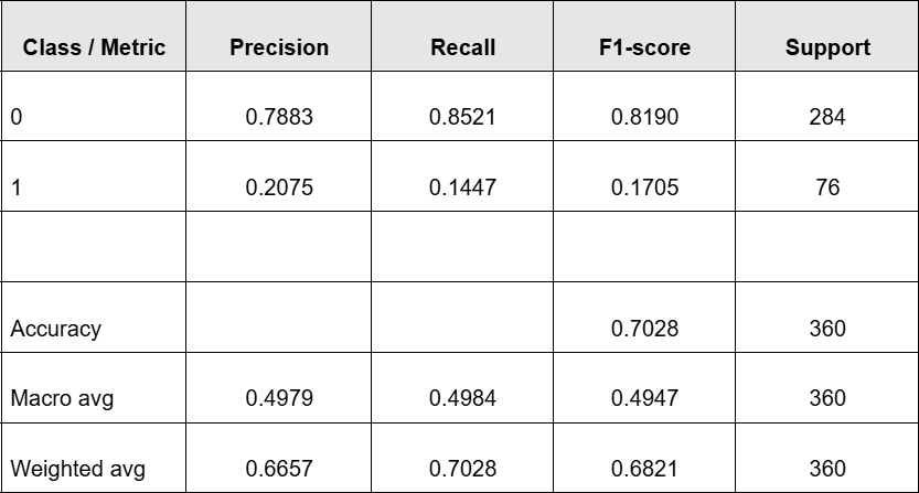
The Output is:
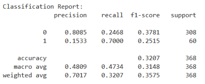
Model Prediciton Backtesting
After obtaining the best prediction results from Random Forest and XGBoost, we wrote the results back to the date labels and attempted to backtest them for trading. Since our prediction target is VIXY price surges, our trading strategy will focus on achieving a significantly high profit-to-loss ratio, disregarding win rate.
Our final trading strategy employs a predictive signal-driven event-based (intraday to overnight) trading framework. First, the model is trained on historical data, with only the out-of-sample prediction results written back to the trading log to avoid look-ahead bias. When the model generates a valid prediction signal (y_pred) on a given trading day, the strategy initiates a position at the t+1 day's opening price (Open_{t+1}). Profit-taking and stop-loss levels are not fixed ratios but dynamically estimated based on the average spike up/down amplitude over the past 20 trading days to capture market volatility structure: the take-profit level is set at 4 times the historical average upward amplitude above the opening price, while the stop-loss level is set at 1 times the historical average downward amplitude below the opening price, creating an asymmetric risk-reward structure. During the holding period, if the lowest price on day t+1 first hits the stop-loss price, the position is closed via stop-loss exit. Otherwise, if the highest price reaches the take-profit price, the position is closed for profit. If neither is triggered, the position is closed at the t+1 closing price. At the same time, if both take-profit and stop-loss orders are triggered simultaneously, we prioritize executing the stop-loss strategy to stress-test our trading model. Final returns are measured by the yield relative to the opening price based on the actual exit price.
Backtesting Result(Random Forest):
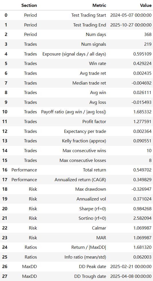
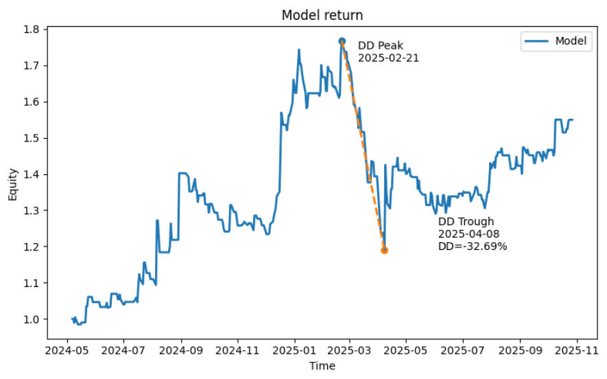
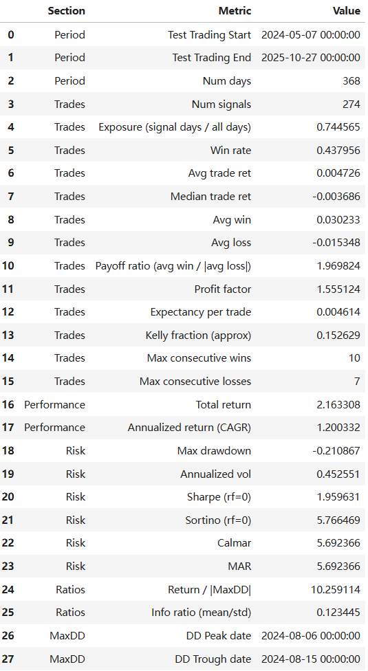
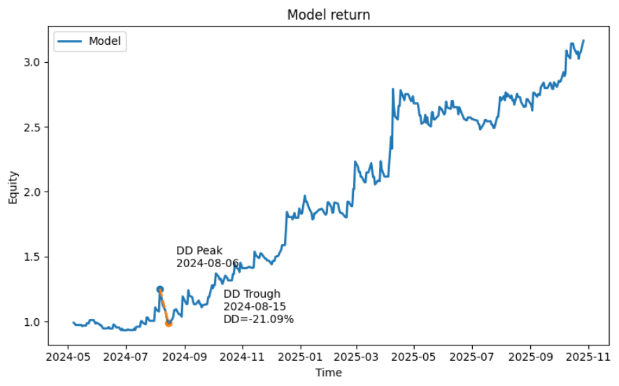
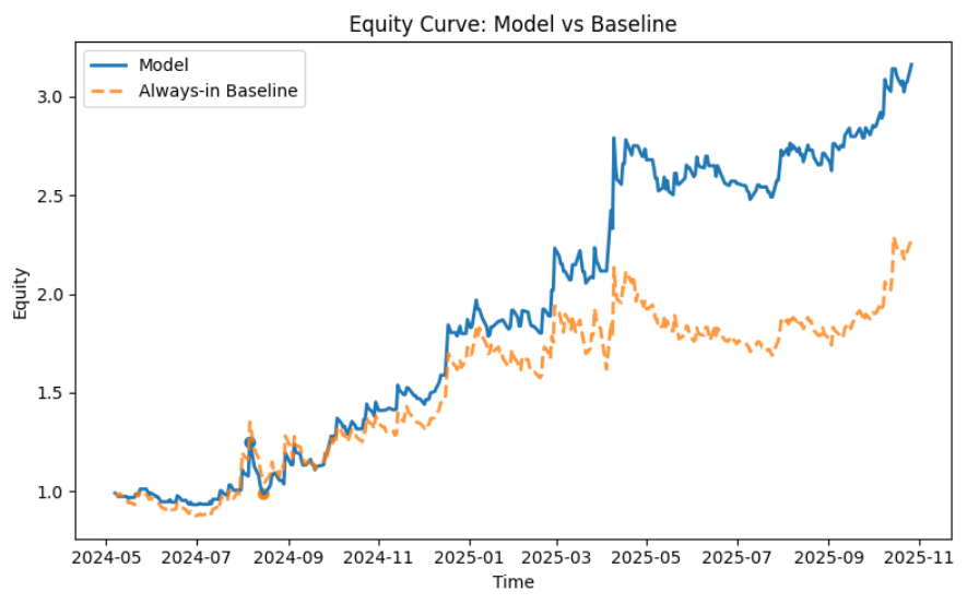
Backtesting Result(XGBoost):
Experimental model: LSTM Neural Network Model
Why LSTM?
Random Forest treats each trading day as an independent observation. However, both volatility and information flow are sequential: market uncertainty can accumulate over days, and tweet narratives can be persistent rather than one-off shocks. Therefore, we use Long Short-Term Memory (LSTM), a recurrent neural network designed to learn temporal dependencies in sequences.
In our implementation, each observation is no longer “one day”, but a sequence window of past days’ embeddings, and the model predicts whether the current day is an abnormal volatility event.
Current Progress
Currently, we hold high expectations for the potential performance of LSTM models. Compared to traditional machine learning methods, LSTMs possess a structural advantage in capturing long-term temporal dependencies within time series data. This characteristic holds promise for significantly enhancing the modeling capability of target variables' dynamic evolution processes, thereby further improving predictive performance. However, uncertainties remain regarding the specific design of LSTM training workflows and the systematic tuning of key hyperparameters—such as network architecture, time window length, and regularization mechanisms. These aspects require further exploration through more in-depth experiments and validation in subsequent research.
References
[1] Yang, Y., Uy, M.C.S. & Huang, A. (2020). FinBERT: A pretrained language model for financial communications. arXiv preprint arXiv:2006.08097.
[2] ProsusAI. (2020). FinBERT. Hugging Face. ProsusAI Accessed 21 January 2026.
[3] Hasan, B.M.S. and Abdulazeez, A.M. (2021) 'A review of principal component analysis algorithm for dimensionality reduction', Journal of Soft Computing and Data Mining, 2(1), pp.20–30.
[4] Breiman, L. (2001) 'Random forests', Machine Learning, 45(1), pp.5–32.