Regression Analysis of Sentiment and Stock Prices (by Group "Semantic Fragments Synthesizer")

Introduction

Every quarter, companies hold earnings calls to report their performance to investors. Does the tone of company leadership—whether optimistic or concerned—genuinely influence stock prices?

We investigated this question within the automotive industry, analyzing over 400 earnings calls from nine major manufacturers, including Tesla, Toyota, and Volkswagen. Our study aimed to answer two key questions:

1. Does a positive sentiment in earnings conference calls correlate with greater stock price increases in the short term versus the long term?
2. How does executive sentiment affect stock price volatility?

1 Methodology

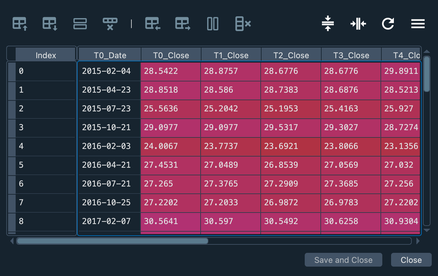
To analyze the impact of earnings calls, we collected stock price data for the five trading days following each call. Using Python and data from Stooq, we extracted daily closing prices for each earnings announcement date (T₀) and the subsequent five trading days (T₁–T₅).

The data collection process automatically adjusts for non-trading days such as weekends and holidays. By modifying only the stock symbol and earnings date list, the same script can gather data for any publicly traded company.

Example: General Motors Data Processing

Here is the Python code used to extract and process General Motors' stock price data:

import pandas as pd
from datetime import datetime, timedelta

# Download General Motors historical data from Stooq
df_gm = pd.read_csv("https://stooq.com/q/d/l/?s=gm.us&i=d")
df_gm['Date'] = pd.to_datetime(df_gm['Date'])
df_gm.set_index('Date', inplace=True)

# Earnings announcement dates for General Motors (2015-2025)
gm_dates = [
    "2015-02-04", "2015-04-23", "2015-07-23", "2015-10-21",
    "2016-02-03", "2016-04-21", "2016-07-21", "2016-10-25",
    "2017-02-07", "2017-04-28", "2017-07-25", "2017-10-24",
    "2018-02-06", "2018-04-26", "2018-07-25", "2018-10-31",
    "2019-02-06", "2019-04-30", "2019-08-01", "2019-10-29",
    "2020-05-06", "2020-07-29", "2020-11-05", "2021-02-10",
    "2021-05-05", "2021-08-04", "2021-10-27", "2022-02-01",
    "2022-04-26", "2022-07-26", "2022-10-25", "2023-01-31",
    "2023-04-25", "2023-07-25", "2023-10-24", "2024-01-30",
    "2024-04-23", "2024-07-23", "2024-10-22", "2025-01-28",
    "2025-05-01", "2025-07-22", "2025-10-21"
]

# Collect stock prices for 5 trading days after each earnings call
gm_data = []

for d in gm_dates:
    target = datetime.strptime(d, "%Y-%m-%d")

    # Adjust for non-trading days
    if target not in df_gm.index:
        before = df_gm.index[df_gm.index <= target]
        if len(before) > 0:
            target = before[-1]  # Use last available trading date
        else:
            continue

    t0_close = df_gm.loc[target, 'Close']

    # Collect closing prices for next 5 trading days
    t_closes = []
    current = target + timedelta(days=1)
    count = 0

    while count < 5:
        if current in df_gm.index:
            t_closes.append(df_gm.loc[current, 'Close'])
            count += 1
        current += timedelta(days=1)

    # Store results
    row = {
        'T0_Date': target.strftime("%Y-%m-%d"),
        'T0_Close': t0_close
    }

    for i in range(5):
        if i < len(t_closes):
            row[f'T{i+1}_Close'] = t_closes[i]

    gm_data.append(row)

# Create DataFrame and save results
gm_df = pd.DataFrame(gm_data)
gm_df.to_csv("gm_result.csv", index=False)
print(f"Processed {len(gm_df)} earnings events for General Motors")

Result：

1.1 Calculating Market Reactions

After obtaining stock prices for the required dates, we proceed to calculate Cumulative Abnormal Returns (CAR) and volatility measures.

companies_reaction = {
    'General Motors': gm_df,
    'Tesla': tsla_df,
    'BMW': bmw_df,
    'Ford': ford_df,
    'Volkswagen': volkswagen_df,
    'Ferrari': ferrari_df,
    'Honda': honda_df,
    'Toyota': toyota_df,
    'Mercedes': mercedes_df
}

reaction_data = []
for name, df in companies_reaction.items():
    # Calculate immediate reaction (T0 to T1)
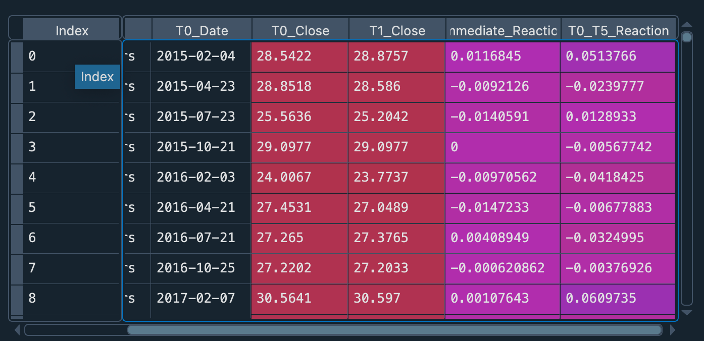
    df['Immediate_Reaction'] = (df['T1_Close'] - df['T0_Close']) / df['T0_Close']

    # Calculate cumulative reaction (T0 to T5)
    df['T0_T5_Reaction'] = (df['T5_Close'] - df['T0_Close']) / df['T0_Close']

    df['Company'] = name
    reaction_data.append(df[['Company', 'T0_Date', 'T0_Close', 'T1_Close', 
                             'Immediate_Reaction', 'T0_T5_Reaction']])

reaction_result = pd.concat(reaction_data, ignore_index=True)
reaction_result.to_csv('Car_Companies_Reaction.csv', index=False)

Result：

1.2 Volatility Analysis

To measure market uncertainty following earnings announcements, we calculated price volatility:

companies_vol = {
    'General Motors': gm_df,
    'Tesla': tsla_df,
    'BMW': bmw_df,
    'Ford': ford_df,
    'Volkswagen': volkswagen_df,
    'Ferrari': ferrari_df,
    'Honda': honda_df,
    'Toyota': toyota_df,
    'Mercedes': mercedes_df
}

vol_data = []
for name, df in companies_vol.items():
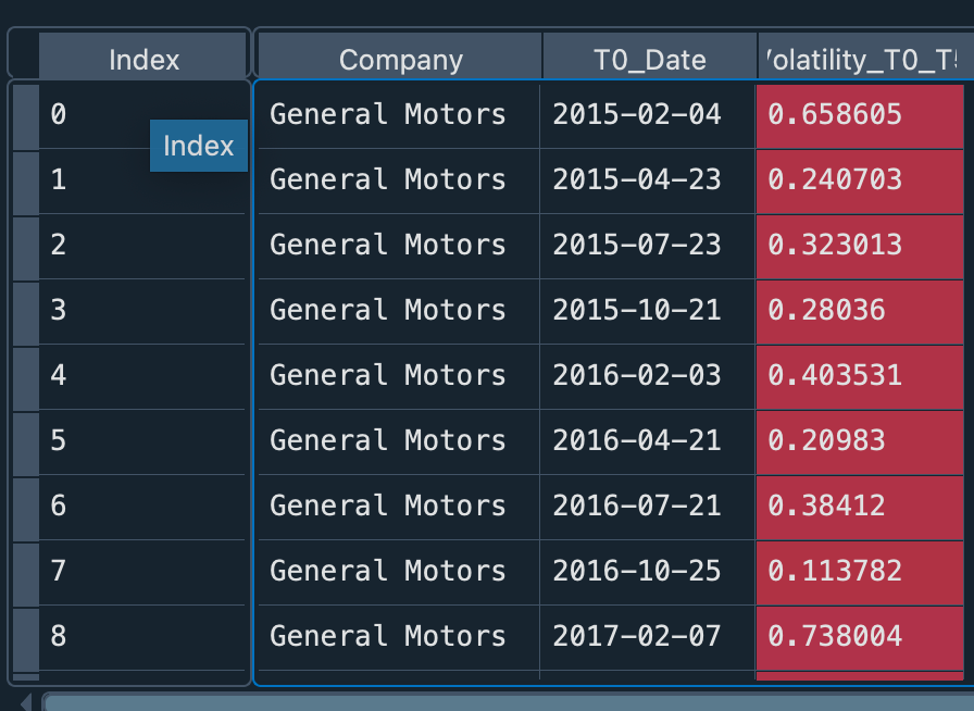
    df['Volatility_T0_T5'] = df[['T0_Close', 'T1_Close', 'T2_Close', 'T3_Close', 'T4_Close', 'T5_Close']].std(axis=1)
    df['Company'] = name
    vol_data.append(df[['Company', 'T0_Date', 'Volatility_T0_T5']])

vol_result = pd.concat(vol_data, ignore_index=True)
vol_result.to_csv('Car_Companies_Volatility.csv', index=False)

Volatility (T₀–T₅): Standard deviation of the six closing prices (T₀ through T₅)

Output: Car_Companies_Volatility.csv, containing company, date, and volatility value

This workflow systematically quantifies the market's price response and uncertainty in the five trading days following earnings calls, enabling further analysis of how earnings‑call sentiment influences short‑term stock behavior.

Result：

2. Sentiment Analysis Methodology

2.1 Objective and Output

Objective : The objective of this step is to compute a call-level baseline sentiment score for each earnings call transcript.

Output (Call-level Table) :

The output is a structured dataset where:

• Each row corresponds to one earnings call

• Each observation represents call-level sentiment, rather than sentence- or word-level sentiment

Key Columns

['company', 'filename', 
 'vader_pos', 'vader_neg', 'vader_neu', 'vader_compound',
 'n_words_full']  # optional: word count

This table provides the foundation for subsequent sentiment comparison and regression analysis.

2.2 Preprocessing Strategy (Key Fix)

Text preprocessing plays a critical role in VADER's performance. We found that over-aggressive cleaning—such as removing punctuation or splitting contractions—can distort VADER's rule-based scoring mechanism.

Example: Transforming "don't" into "don t" weakens negation handling and may bias sentiment scores upward.

To address this issue, we adopt a dual preprocessing strategy:

# Strategy 1: Light preprocessing for VADER
# Preserves negations and punctuation cues essential for rule-based scoring

# Strategy 2: Heavier preprocessing for dictionary-based methods (e.g., LM)
# Removes punctuation and contractions not required for these methods

This separation ensures that each sentiment method operates on text that is appropriate for its underlying assumptions.

import re

# Light cleaning for VADER: preserve negations and punctuation cues
def clean_for_vader(text: str) -> str:
    text = text.replace("\u00a0", " ")
    text = re.sub(r"\s+", " ", text).strip()
    return text

# Heavier cleaning (optional): useful for dictionary counting (e.g., LM)
def clean_for_lm(text: str) -> str:
    text = text.lower()
    text = re.sub(r"[^a-z\s]", " ", text)
    text = re.sub(r"\s+", " ", text).strip()
    return text

2.3 Call-level Scoring with VADER

Using the lightly preprocessed transcripts, we compute VADER sentiment at the call level, treating each earnings call as a single observation. Sentiment scores are obtained via the polarity_scores() function, with the compound score serving as the primary baseline sentiment measure.

The implementation iterates through company folders and transcript files, applies VADER scoring, and stores the results in a call-level dataset.

Code: iterate through folders and compute VADER scores

rows = []

for company in os.listdir(FOLDER):
    company_path = os.path.join(FOLDER, company)
    if not os.path.isdir(company_path):
        continue

    for file in os.listdir(company_path):
        if not file.lower().endswith(".txt"):
            continue

        file_path = os.path.join(company_path, file)
        with open(file_path, "r", encoding="utf-8", errors="ignore") as f:
            raw = f.read()

        vader_input = clean_for_vader(raw)
        scores = sid.polarity_scores(vader_input)

        rows.append({
            "company": company,
            "filename": file,
            "vader_pos": scores["pos"],
            "vader_neg": scores["neg"],
            "vader_neu": scores["neu"],
            "vader_compound": scores["compound"],
            "n_words_full": len(clean_for_lm(raw).split())  # optional
        })

Key Features:

1. Call-level analysis: Each earnings call treated as a single observation
2. Dual preprocessing: Uses clean_for_vader() for sentiment scoring, clean_for_lm() for word counting
3. Comprehensive output: Captures all four VADER sentiment dimensions (positive, negative, neutral, compound)
4. Flexible storage: Results can be easily converted to DataFrame for further analysis

Output Structure:

The resulting dataset contains sentiment scores for each earnings call, ready for correlation with stock price reactions calculated in Section 1.

2.4 Role in the Overall Pipeline

VADER sentiment provides a general-purpose baseline measure of managerial tone. In later steps, this baseline is compared with finance-specific sentiment measures derived from the Loughran–McDonald dictionary and related to market reactions (CAR) through regression analysis. This design allows us to distinguish broad emotional tone from economically meaningful sentiment.

2.5 Distribution of VADER Sentiment Scores

To assess the overall behavior of VADER sentiment across earnings calls, we examine the distribution of VADER compound scores. This visualization provides a descriptive overview of sentiment dispersion and helps identify potential clustering or extreme values.

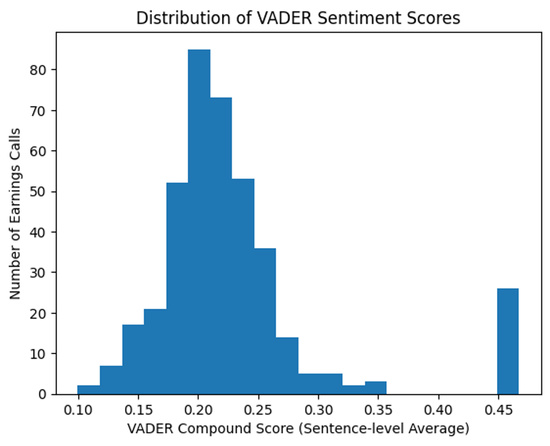
The distribution shows that most VADER compound scores are concentrated in a narrow, mildly positive range, with few extreme observations. This pattern is consistent with the professional and institutional nature of earnings call communication and supports the interpretation of VADER as a baseline tone indicator rather than a measure of strong emotional expression.

Key Takeaways from the Distribution

• Concentration around low positive values
• Absence of extreme sentiment scores
• Consistency with neutral, institutional disclosure language
• Support for VADER as a baseline sentiment benchmark

How This Fits into the Analysis

This distributional evidence motivates the use of finance-specific sentiment measures in subsequent analysis. While VADER captures overall tone, it may not fully reflect economically meaningful sentiment embedded in financial terminology. This limitation is addressed in the next section using the Loughran–McDonald dictionary.

3. LM Financial Dictionary Tone for Earnings Calls (Automakers)

3.1 What We Built in This Milestone

In this milestone, we built Loughran–McDonald (LM) financial dictionary sentiment features for each earnings call transcript. The goal is to turn raw transcripts into interpretable, finance-aware tone ratios, which can be merged with event dates and stock return data later.

For each transcript, the output includes: - Basic identifiers (firm, filename, call_id, call_date, year/quarter) - Transcript length (word_count) - LM counts and length-normalized ratios (Positive / Negative / Uncertainty) - Additional derived measures (net tone, tone strength)

3.2 Load the Official LM Dictionary and Build Word Sets

We use the official LM Master Dictionary (1993–2024) CSV file and convert it into three word sets: Positive, Negative, and Uncertainty. This makes counting fast: for each token, we just check membership in a set.

lm = pd.read_csv(LM_CSV)
lm["Word"] = lm["Word"].astype(str).str.lower()

POS_SET = set(lm.loc[lm["Positive"] > 0, "Word"])
NEG_SET = set(lm.loc[lm["Negative"] > 0, "Word"])
UNC_SET = set(lm.loc[lm["Uncertainty"] > 0, "Word"])

print("[INFO] LM sizes:", len(POS_SET), len(NEG_SET), len(UNC_SET))

3.3 Clean transcripts into consistent tokens

To make dictionary matching reliable, we apply a simple cleaning function:

• lowercase

• keep only letters and whitespace

• collapse multiple spaces

This is a trade-off: it improves robustness and speed, but it ignores context (e.g., negation) because LM is dictionary-based.

def clean_text(text: str) -> str:
    text = text.lower()
    text = re.sub(r"[^a-z\s]", " ", text)
    text = re.sub(r"\s+", " ", text).strip()
    return text

3.4 Robust call date parsing (the unicode dash issue)

A practical problem: transcript filenames often include dates, but sometimes the dash in filenames is not the normal ASCII -.

It can be an en-dash (–) or other unicode dash characters. Visually they look the same, but regex matching fails.

We solved this by normalizing unicode in filenames first, converting different dash characters to -, then extracting the YYYY-MM-DD pattern.

def normalize_filename(s: str) -> str:
    s = unicodedata.normalize("NFKC", s)
    for ch in ["\u2013", "\u2014", "\u2212", "\uFF0D"]:
        s = s.replace(ch, "-")
    return s

def parse_call_date(filename: str):
    fn = normalize_filename(filename)
    m = re.search(r"(?<!\d)(20\d{2})[-_](\d{2})[-_](\d{2})(?!\d)", fn)
    if not m:
        return None
    return datetime(int(m.group(1)), int(m.group(2)), int(m.group(3))).strftime("%Y-%m-%d")

3.5 Count LM Words and Compute Ratios (Length Normalization)

For each transcript:

• Tokenize → get word_count

• Count LM matches: lm_pos_cnt, lm_neg_cnt, lm_unc_cnt

• Convert counts to ratios by dividing by total words

Ratios are important because earnings calls have very different lengths. Without normalization, longer calls would mechanically have larger counts and bias comparisons.

We also compute:

• lm_net_tone = lm_pos_ratio − lm_neg_ratio

• lm_tone_strength = lm_pos_ratio + lm_neg_ratio

pos_cnt = sum(1 for t in tokens if t in POS_SET)
neg_cnt = sum(1 for t in tokens if t in NEG_SET)
unc_cnt = sum(1 for t in tokens if t in UNC_SET)

pos_ratio = pos_cnt / word_count
neg_ratio = neg_cnt / word_count
unc_ratio = unc_cnt / word_count

lm_net_tone = pos_ratio - neg_ratio
lm_tone_strength = pos_ratio + neg_ratio

4. VADER Regression: Baseline Evidence

To move beyond descriptive sentiment analysis, we first examine whether overall earnings call sentiment, as measured by VADER, is associated with short-term market outcomes.

We estimate a baseline regression linking VADER sentiment to two dimensions of market response: price reactions, measured by cumulative abnormal returns (CAR) over T0–T1 and T0–T5, and market uncertainty, measured by post-call stock price volatility over T0–T5.

The results show no statistically significant relationship between VADER sentiment and CAR under both linear and nonlinear specifications. This suggests that the general tone of earnings calls does not systematically drive short-term price movements, as earnings-related information is already anticipated and incorporated into prices before the call.

In contrast, VADER sentiment exhibits a strong, statistically significant negative relationship with post-call volatility. More positive earnings call sentiment is associated with lower subsequent stock price volatility, with an estimated coefficient of −4.22 (p < 0.001). This finding indicates that managerial tone may help reduce market uncertainty, even when it does not trigger immediate price changes.

Overall, these results suggest that VADER captures a general tone effect in earnings calls. While informative, this broad sentiment measure does not distinguish between economically meaningful types of language. We therefore turn to a finance-specific dictionary approach in the next section to provide a more granular interpretation of how earnings call language relates to market reactions.

5. Loughran–McDonald Dictionary: Finance-Specific Evidence on Volatility

While the VADER analysis provides useful baseline evidence, it relies on a general-purpose sentiment measure that treats all positive or negative language equally. However, earnings calls are highly specialized financial communications, where words such as “risk,” “uncertain,” “expects,” or “challenging” carry meanings that may not be well captured by general sentiment tools.

To address this limitation, we turn to the Loughran–McDonald (LM) financial dictionary, which is specifically designed for corporate disclosures. This allows us to distinguish between overall optimism and uncertainty-related language, both of which may affect investors in different ways.

Using the LM dictionary, we construct three key sentiment variables for each earnings call:

Net Tone: the difference between positive and negative word ratios

Net Tone Squared: to capture potential non-linear effects

Uncertainty Ratio: the share of uncertainty-related words in the transcript All measures are normalized by transcript length to ensure comparability across calls of different sizes.

We then re-estimate the same regression framework used in the VADER analysis, focusing on three market outcomes: immediate returns, short-horizon cumulative returns (CAR), and post-call volatility.

-OLS regression function:

def run_ols_export(y_var, X_vars, data, output_file):
    df_reg = data.dropna(subset=[y_var] + X_vars)

    print(f"\nRunning regression for {y_var}, N = {len(df_reg)}")

    X = sm.add_constant(df_reg[X_vars])
    y = df_reg[y_var]

    model = sm.OLS(y, X).fit(cov_type="HC3")
    print(model.summary())

    summary_df = pd.DataFrame({
        "coef": model.params,
        "std_err": model.bse,
        "t": model.tvalues,
        "p_value": model.pvalues,
        "conf_lower": model.conf_int()[0],
        "conf_upper": model.conf_int()[1]
    })

    extra = pd.DataFrame({
        "coef": [len(df_reg), model.rsquared]
    }, index=["N", "R_squared"])

  summary_df = pd.concat([summary_df, extra])
    summary_df.to_excel(output_file)

    print(f"Results exported to {output_file}")
    return model

This function runs an OLS regression with HC3 robust standard errors, prints the regression summary, and exports a compact results table including coefficients, t-statistics, p-values, confidence intervals, sample size, and R².

Running regressions for three market outcomes:

X_vars = ["lm_net_tone", "lm_net_tone_sq", "lm_unc_ratio"]

y_vars = {
    "Volatility_T0_T5": r"C:\Users\18443\Desktop\Reg_Volatility.xlsx",
    "Immediate_Reaction": r"C:\Users\18443\Desktop\Reg_Immediate_Reaction.xlsx",
    "T0_T5_Reaction": r"C:\Users\18443\Desktop\Reg_T0_T5_Reaction.xlsx"
}

models = {}
for y_var, out_file in y_vars.items():
    if y_var not in df.columns:
        print(f"Skipping {y_var} (not found)")
        continue
    models[y_var] = run_ols_export(y_var, X_vars, df, out_file)

Result

First, earnings call sentiment measured by the LM dictionary does not predict stock returns, either immediately or over the T0–T5 window. Both linear and non-linear sentiment terms are insignificant, and the return regressions exhibit very low explanatory power. This indicates that managerial language does not systematically affect short-term price direction, consistent with rapid incorporation of return-relevant information into prices.

Second, LM sentiment shows a strong and economically meaningful relationship with post-earnings volatility. Net tone enters positively, while its squared term enters negatively, implying a clear inverted U-shaped relationship. Moderate optimism is associated with higher volatility, whereas extremely positive and confident language is linked to lower volatility.

In addition, the uncertainty ratio is a robust positive predictor of volatility. Earnings calls containing more uncertainty-related language are followed by significantly higher stock price volatility, even after controlling for overall tone. Overall, the LM dictionary reveals that while sentiment does not generate return predictability, finance-specific language—particularly uncertainty—plays a central role in shaping post-announcement risk and investor disagreement.