By Group "Deepsick"
Introduction
This project aims to predict future interest rate decisions by analyzing the text of Federal Open Market Committee (FOMC) statements. In our previous post, we detailed the data acquisition and preprocessing pipeline for this project. Our dataset collects FOMC statements from 2000 to 2025, each paired with subsequent shifts in the effective federal funds rate. These statements were categorized into three labels: rate increase (1), neutral (0), and rate decrease (−1). Following text normalization and lemmatization, we extracted 1,383 TF-IDF features using a combination of unigrams and bigrams. In this blog, we will focus on dataset split, model training, and hyperparameter optimization, concluding with a comprehensive analysis of our predictive results.
Data Split
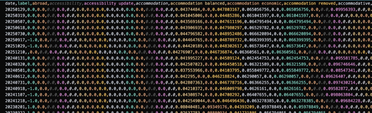
The table below presents the final dataset constructed in our previous blog. The target variable Y is a three-class label indicating policy direction, taking values −1, 0, and 1, while the input features X consist of TF-IDF based textual representations. The full dataset contains 219 observations (already removed last observation without label) and 1,383 features, generated using unigram and bigram configurations.
We proceed to prepare the data for model training by applying a time-based data split, which better reflects real-world forecasting settings.
# 2000 - 2016: training set
   train_df = df[df["date"] < CUTOFF1]
   # 2017 - 2020: validation set
   valid_df = df[(df["date"] >= CUTOFF1) & (df["date"] < CUTOFF2)]
   # 2021 - 2025: test set
   test_df = df[df["date"] >= CUTOFF2]
Specifically, the training set consists of 145 observations from 2000 to 2016, the validation set includes 35 observations from 2017 to 2020, and the test set contains 39 observations from 2021 to 2025.
A potential limitation of this split is that different time periods correspond to distinct macroeconomic regimes. For instance, years such as 2001 and 2003 are associated with economic downturns, while 2002 and 2004 reflect recovery phases. As a result, the economic environments represented in the training and test sets may differ substantially, which can introduce bias in model predictions. To mitigate this issue, we employ a Random Forest model in the following steps. It reduces variance by constructing multiple decision trees from randomly sampled subsets of the training data and aggregating their predictions, thereby improving robustness across varying economic conditions.
Support Vector Machine (SVM)
Building on our processed dataset, we first apply a linear Support Vector Machine (SVM) to predict policy rate movements from FOMC statement text. Linear SVMs are well suited for text classification tasks due to their effectiveness in high-dimensional and sparse feature spaces. The model is implemented using LinearSVC from scikit-learn with a one-vs-rest strategy to handle the three-class setting. To address potential class imbalance, class-weighted loss is applied.
The key hyperparameter of the linear SVM is the regularization parameter C, which controls the trade-off between fitting the training data and maintaining generalization. We tune C using the validation set, selecting the value that maximizes macro-averaged F1 score. Macro-F1 is chosen over accuracy because it weights each policy outcome equally and is therefore more appropriate in a multi-class, imbalanced setting.
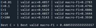
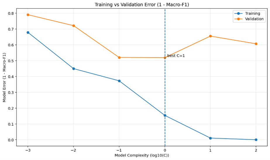
Among candidate values C∈{0.01,0.1,1,10,100}, the model achieves the highest validation macro-F1 at C=1, which is selected as the final specification. The accompanying figure shows that while training error decreases monotonically as C increases, validation error follows a U-shaped pattern, reflecting a bias–variance trade-off. The minimum validation error occurs at C=1, supporting this choice.
After selecting the optimal hyperparameter, we refit the SVM on the combined training and validation data. On this in-sample dataset, the model achieves an accuracy of 0.87 and a macro-F1 score of 0.86, indicating a strong fit. Performance is high across all three classes, suggesting that the SVM can effectively separate policy outcomes within the sample period.
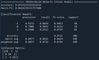
We then evaluate the model on the held-out test set covering 2021–2025. Out-of-sample performance declines, with an accuracy of 0.67 and a macro-F1 score of 0.68, which is expected given the limited sample size and structural changes in the macroeconomic environment. Notably, the model performs best in identifying rate increases, achieving perfect precision and high recall for this class. Performance for no-change decisions is moderate, while rate decreases are more difficult to predict, with lower precision due to overlap in accommodative and neutral policy language.
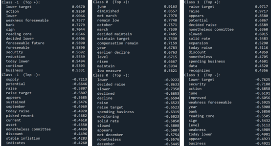
To interpret the model’s predictions, we examine the most influential features for each class. For rate decreases, highly weighted terms include phrases such as “lower target” and “reduction,” reflecting accommodative policy signals. The no-change class is associated with phrases like “decided maintain” and “maintain target,” while rate increases are strongly linked to terms such as “raise,” “raise target,” and language indicating economic strength. These patterns align closely with economic intuition and demonstrate the interpretability of the linear SVM.
Overall, while the SVM exhibits a clear generalization gap between in-sample and test performance, it provides a strong and interpretable baseline for predicting monetary policy actions from FOMC statements textual data.
Random Forest Model
Following the evaluation of the Support Vector Machine (SVM) model, we further applied a Random Forest model to predict the direction of changes in the federal funds rate. As an ensemble learning method, Random Forest reduces the risk of overfitting and typically handles high-dimensional feature spaces effectively by constructing multiple decision trees and combining their predictions. Unlike linear models, Random Forest can capture nonlinear relationships between features, which may offer an advantage in recognizing complex linguistic patterns within text data.
3.1 Model Implementation and Parameter Settings
We implemented the Random Forest model using the RandomForestClassifier from the scikit-learn library. To address the high dimensionality and sparsity of the TF-IDF feature space, as well as the potential class imbalance among the three labels (rate decrease, unchanged, rate increase), we adopted the following configuration:
Number of Decision Trees: Set to 100 to balance model complexity and computational efficiency.
Class Weights: The 'balanced' parameter was used to automatically adjust class weights, giving higher importance to minority classes.
Feature Selection Strategy: The number of features considered for splitting at each decision tree node was set to the square root of the total number of features ('sqrt'), facilitating the handling of high-dimensional text features.
Randomness Control: random_state=42 was set to ensure reproducibility of the results.
3.2 Model Performance
On the training set, the Random Forest model demonstrates a perfect fit with an accuracy of 0.87.

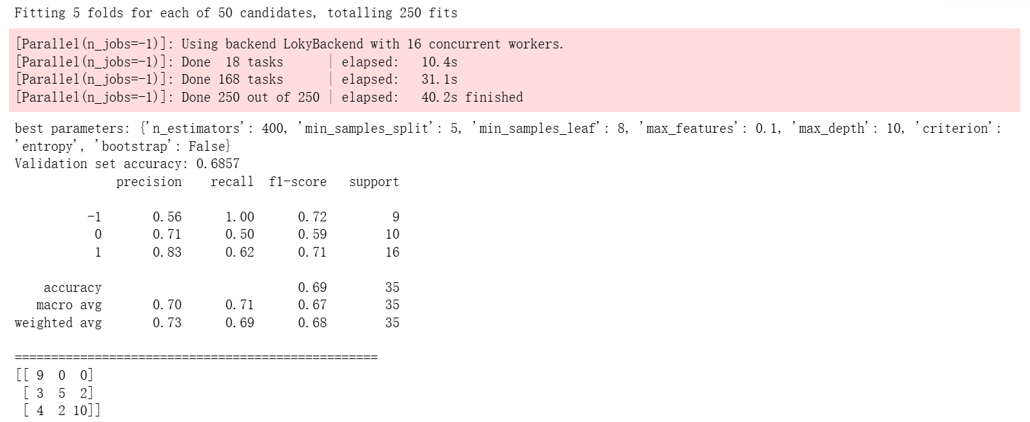
Then, we use the validation data for random forest parameter tuning to obtain the optimal parameters and make predictions on the validation set data, achieving an accuracy of 0.69.
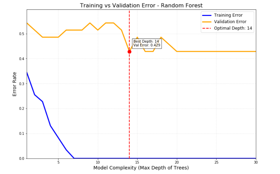
The graph below shows how the errors of a Random Forest model on the training set and validation set change with model complexity (the maximum depth of the trees). As the tree depth increases, the training error continuously decreases and approaches zero, while the validation error first decreases and then rises, reaching its lowest point at a depth of 14, where the model achieves the best generalization ability. When the depth is less than 14, the model is underfitted (both errors are high); when the depth exceeds 14, the model is overfitted (the training error is very low, but the validation error increases). This graph is created to visualize the bias-variance trade-off, help determine the optimal hyperparameters, avoid underfitting or overfitting, and ensure that the model performs well on new data.
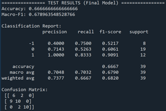
Considering that the model, despite using optimal parameters, achieved a low accuracy in predicting the validation set—particularly for neutral samples—the threshold adjustment method was adopted to enhance the model's predictive capability for the category of unchanged interest rates. The evaluation results on the test set show that the Random Forest model achieves an accuracy of 0.72
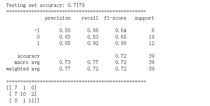
"Rate Increase (+1)" Category: recall = 0.92 — The model captured 92% of the actual rate hike events. Among all cases predicted by the model as "rate increase", 85% were correct.
"Rate Decrease (-1)" Category: recall = 0.88 — The model captured 88% of the actual rate cut events, showing strong performance. In terms of precision, among all cases predicted as "rate decrease," only 50% were correct, with the rest being misclassifications.
"Unchanged (0)" Category: recall = 0.53 — The model only captured 53% of the actual rate remain events. In terms of precision, among all cases predicted as "rate remain," 83% were correct.
Logistic Regression Model
The following are the application of Logistic regression in Python to predict future policy rate movements by using the text in FOMC statements and access the effectiveness and accuracy of the model.
The code completely follows the following modeling logic:
(1) Dataset Division: Training Set (Train) → Parameter Tuning (Validation) → Final Evaluation (Test).
(2) Model Training: Using L2 regularized logistic regression.
(3) Hyperparameter Tuning: Finding optimal regularization strength C through grid search.
(4) Final Evaluation: Evaluating final model performance on test set.
For Train Set, Validation Set and Test Set, we extract and separate features and labels from data frame in data preprocessing section. More importantly, we combine Train Set and Validation Set into a new set called Combined Set for follow-up model training.
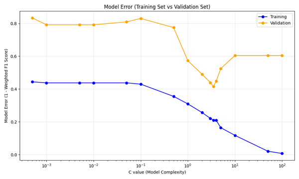
We apply default L2 regularization to search for the best hyperparameter C-value for final model training. To find the best C-value, we construct a list of C_canditates including all regularization strength C-value candidates and covering multiple orders of magnitude. Then we use for-loop to iterate them 5000 times to train primary model on Training Set. The function “accuracy_score” is used to evaluate and select the best C-value whose model performs the best on Validation Set, while the other function “f1_score” is used to evaluate model error for each C-value on Training Set and Validation Set. The result shows the best C-value is 3.5, with the validation accuracy of 0.6.
C_candidates = [0.0005, 0.001, 0.005, 0.01, 0.05, 0.1, 0.5, 1.0, 2.0, 3.0, 3.5, 4.0, \
                5.0, 10.0, 50.0, 100.0]

best_score = -1.0
best_C = None

# Lists to store errors for training set and validation set
train_errors = []
valid_errors = []

for c in C_candidates:
    model = LogisticRegression(
        C=c,
        solver='lbfgs',  # Use L-BFGS optimization algorithm
        max_iter=5000,  # Ensure model convergence (due to high feature dimensionality)
        class_weight='balanced',  # Handle class imbalance
        random_state=42,
        tol=1e-4
    )

    model.fit(X_train, y_train)  # Train model on training set
    score = accuracy_score(y_valid, model.predict(X_valid))

    print(f"C = {c:10.4f}  →  Validation Accuracy: {score:.4f}")

    if score > best_score:
        best_score = score
        best_C = c

    # Calculate weighted F1 for training set and validation set
    # Convert to 1 - F1 as Model Error
    f1_train = f1_score(y_train, model.predict(X_train), average='weighted')
    f1_valid = f1_score(y_valid, model.predict(X_valid), average='weighted')
    train_errors.append(1 - f1_train)
    valid_errors.append(1 - f1_valid)

print(f"\nBest C value: {best_C:.4f}  (Validation Accuracy: {best_score:.4f})\n")
We plot the relationship between model error for Training/Validation Set and model complexity (which is C-value) to judge whether the models of different C-value are overfitting. As the plot below, the best predictive model is obtained at the minimum of the validation error, whose C-value is 3.5.
Then we use the found optimal C-value to train the final model. Considering the scale of Training Set, in order to enhance the effectiveness and accuracy of the final model, we employ Combined Set (Training Set + Validation Set) instead of Training Set to train it.
# Create final model using the found optimal C value
final_model = LogisticRegression(
    C=best_C,
    solver='lbfgs',
    max_iter=5000,
    class_weight='balanced',
    random_state=42,
    tol=1e-4
)

# Train final model using training set + validation set
final_model.fit(X_combined, y_combined)
We define a function called “print_evaluation” to assess effectiveness and accuracy of the final model by using multiple evaluation metrics such as accuracy_score (accuracy), precision_score (precision), recall_score (recall), f1_score (F1 score) and roc_auc_score (ROC area under curve). Then we use it for both Validation Set and Test.
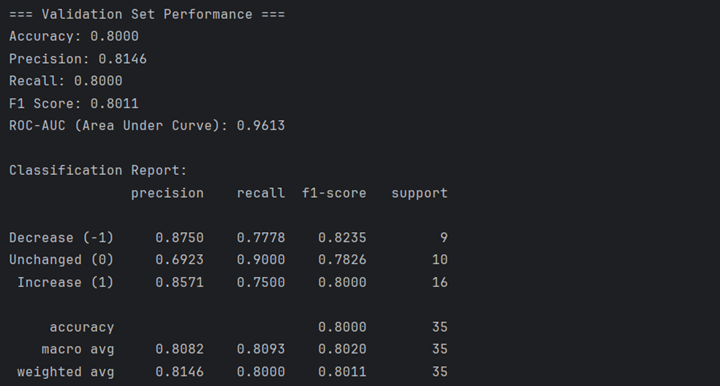
The following shows the performance of final model on the Validation Set. The overall accuracy is 0.8000, which meets our expectations. The prediction of final model is well performed on the decrease and the increase of EFFR. However, it has relatively poor performance when EFFR is unchanged, with the accuracy of 0.6923. This means that the final model is probably not stable when forecasting unchanged EFFR, despite the small scale of Validation Set.
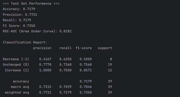
The following shows the performance of final model on the Test Set. The overall accuracy is 0.7179, which is lower than that on the Validation Set but also acceptable. The prediction of final model is absolutely correct on the increase of EFFR and relatively well performed when the EFFR unchanged. However, it performs worse when EFFR decreases, with the accuracy of 0.4167, slightly better than random guess. The performance of the final model on the Test Set is obviously different from that on Validation Set, which indicates that the final model is not stable enough for precise prediction.
From my perspective, there are several reasons that account for the different results on the two data set. First, logistic regression itself is not suitable for the project if the data has complex, non-linear relationship. Second, the scale of the three data set is too small for machine learning and model training, which results in the instability of the final model. Last but not least, the construction of the two data set may be unreasonable. These three data set cover different years. As different years have different characteristics in several aspects such as economic performance, the attribute of the data in different data sets may have a large difference, which influences modeling.
Overall, despite the limitations we mention above, the logistic regression model is relatively suitable for EFFR forecasting.
Model Comparison
To better understand the relative strengths and limitations of different modeling approaches, we compare the out-of-sample performance of the three classifiers used in this project: Logistic Regression, Support Vector Machine (SVM), and Random Forest. All models are trained using the same TF-IDF feature set and evaluated on a common held-out test period from 2021 to 2025, ensuring a fair comparison.
Overall, Random Forest achieves the highest test accuracy (approximately 72%) after threshold adjustment, reflecting its ability to capture nonlinear relationships in the text data. However, this performance comes at the cost of reduced interpretability and a tendency to overfit the training data, as evidenced by its near-perfect in-sample fit.
Logistic Regression delivers competitive test performance (around 71–72%), while maintaining strong interpretability. Its linear structure allows clear identification of economically meaningful keywords associated with rate hikes and cuts. Nevertheless, its performance varies noticeably across time periods, suggesting sensitivity to structural changes and limited capacity to model nonlinear text–policy relationships.
The linear SVM provides a strong and interpretable text-classification benchmark, with solid in-sample performance and reasonable out-of-sample accuracy (around 67%). However, its generalization deteriorates in the most recent test period, particularly for neutral policy decisions, highlighting challenges associated with temporal language drift and regime changes.
Across all models, a consistent pattern emerges: rate increases and rate decreases are predicted more reliably than no-change decisions. This reflects the inherently ambiguous and context dependent nature of neutral policy language in FOMC statements, which remains difficult for frequency-based text models to capture.
Summary
This project develops an end-to-end text-based framework for Fed watching, transforming qualitative FOMC communications into quantitative signals and evaluating their predictive power for future interest rate decisions. Using TF-IDF representations of FOMC statements from 2000 to 2025 and a time-aware train–validation–test split, we systematically assess the performance of Logistic Regression, SVM, and Random Forest models.
Our results demonstrate that FOMC language does contain economically meaningful information related to future policy actions, particularly for directional decisions such as rate hikes and cuts. At the same time, the analysis highlights important limitations. Model performance is sensitive to sample size, macroeconomic regime shifts, and changes in policy communication style over time. In particular, predicting policy inertia (“no change”) remains challenging across all approaches.
Taken together, these findings suggest that while text-based models provide a useful and interpretable baseline for monetary policy analysis, no single model or signal dominates consistently across periods. This reinforces the importance of incorporating regime awareness and complementary strategies when applying NLP techniques to real-world Fed watching and policy forecasting tasks.