Predicting Federal Funds Rate Movements from FOMC Statement(by Group "Deepsick")

By Group "Deepsick"

Introduction

Monetary policy communication plays an important role in shaping market expectations, with the Federal Funds Rate being one of the most closely watched policy indicators. Although the Federal Open Market Committee (FOMC) communicates its decisions through official statements and meeting minutes, these texts are qualitative in nature and difficult to interpret systematically.

Recent advances in natural language processing (NLP) make it possible to transform such unstructured text into quantitative features. This project explores whether the language used in FOMC communication contains predictive signals about future movements in the Federal Funds Rate.

This project explores whether NLP techniques can be used to extract quantitative signals from FOMC communication and assess whether policy language contains information about future movements in the Federal Funds Rate. The textual analysis is linked to observed interest rate outcomes using data from Federal Reserve Economic Data (FRED).

By framing monetary policy prediction as a text-based classification problem, this project provides a practical demonstration of how relatively simple NLP techniques can be applied to real-world policy documents.

Data Source

1. FOMC text data:

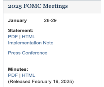
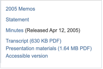
The textual data consist of FOMC statements and meeting minutes collected from official Federal Reserve websites. The we use FOMC Calendars to obtain documents from recent years (2020–2025), while the FOMC Historical Year to collect documents from earlier years (2000–2019).

In total, the dataset includes:

• 220 FOMC statements
• 207 FOMC meeting minutes
• Coverage period: 2000–2025

2. Monetary Policy Data:

The effective federal funds rate (DFF) data are obtained from FRED. In total, the dataset includes:

• 9,497 daily observations.
• Coverage period: 2000–2025

In the following section, we introduce the data preprocessing procedures and corresponding strategies.

Step 1: Data Collection

For the text data, firstly we import the libraries. Since the Federal Reserve’s website is static, which does not require the user interaction or JavaScript rendering, we conduct the Requests library to do the web scraping.

import requests
from bs4 import BeautifulSoup
import re
import pandas as pd
from datetime import datetime

We download and store the statement and minutes’ html from the current url and history url. Our HTTP requests are sent using the requests library with a standard browser user-agent header to avoid access restrictions. Later, the HTML content is parsed using BeautifulSoup.

headers = {"User-Agent": "Mozilla/5.0"}
# get current html links
response = requests.get(current_url, headers=headers)
soup = BeautifulSoup(response.text, "html.parser")
# get historical html links
hist_response = requests.get(historical_url, headers=headers)
hist_soup = BeautifulSoup(hist_response.text, "html.parser")

Due to inconsistencies in webpage design across different periods, the structure of FOMC pages differs between current and historical URLs.

For recent years, FOMC statements have been published as press releases with standardized HTML structures, allowing statement links to be identified directly through consistent URL patterns. In contrast, historical pages embed statements within year-specific archives alongside various related materials. Statement links are therefore identified using keyword matching (e.g., “statement”) and filtered by the presence of an eight-digit date pattern (YYYYMMDD) in the URL. PDF files and supplementary documents are excluded to avoid irrelevant or duplicate content. Accordingly, separate extraction rules are applied to current and historical pages to ensure consistent and accurate data collection over time.

# 2020-2025 Statement Link
       if (
           text == "HTML"
           and href.startswith("/newsevents/pressreleases/monetary")
           and href.endswith(".htm")
       ):
# 2000-2019 Statement Link
           if (
               2000 <= year <= 2019
               and "statement" in label
               and re.search(r"\d{8}", href)
               and not href.endswith(".pdf")
           ):

Combine the html from 2000-2025 together.

# 3. combine the links of statements and minutes (2000-2025)
   sta_links = statement_links + historical_statement_links
   min_links = minutes_links + historical_minutes_links

Next, we use the beautiful soup to extract the date and text from the HTML. We found that each HTML link contains the meeting date, which was extracted directly from the URL. This approach is more efficient than parsing the date from the HTML content, as the webpage structure is inconsistent across years and makes the date difficult to locate programmatically.

# 4. extract date and text from html
def extract_date_from_url(url: str) -> str:
   """Extract YYYYMMDD from URL only; return empty string on failure."""
   m = re.search(r"(\d{8})", url)
   if not m:
       return ""
   dt = datetime.strptime(m.group(1), "%Y%m%d")
   return dt.strftime("%Y%m%d")

The text content is extracted using the function extract_text_from_soup. Specifically, the function first targets the main content area identified by the col-sm-8 "div", and falls back to "table" elements when necessary. All relevant "p" tags are collected and concatenated to form the complete document text.

Besides, a text-cleaning step is then applied to normalize whitespace. Specifically, carriage returns (\r), line breaks (\n), and tab characters (\t) are replaced with spaces, and multiple consecutive spaces are collapsed into a single space. This ensures a clean and consistent text format for subsequent analysis.

# 5. data cleaning
def data_cleaning(text: str) -> str:
   """
   Normalize whitespace (remove \\r, \\n, \\t) and collapse multiple spaces.
   """
   # Replace common control characters with spaces
   cleaned = text.replace("\r", " ").replace("\n", " ").replace("\t", " ")
   # Collapse repeated spaces
   cleaned = re.sub(r"\s+", " ", cleaned)
   return cleaned.strip()

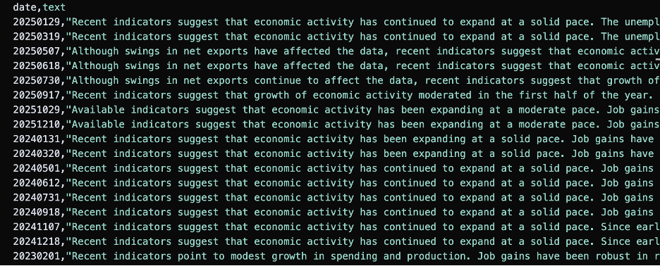
At the end of the data collection process of the text data, we save the date and text into a CSV file. The following shows the resulting statement dataset.

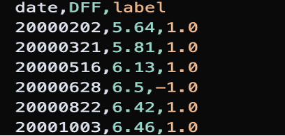
For the DFF data, observations are matched to FOMC statements by date. A policy direction label is constructed as follows:

• +1: rate increase
• 0: no change
• −1: rate decrease

Since rate changes occur after statement releases, the label at time t is defined using the rate movement between t and t+1. The following shows the clean and transformed DFF dataset:

Step 2: Data Preprocessing

In this section, we construct a standard Natural Language Processing (NLP) preprocessing pipeline to transform raw textual data into a clean, structured format suitable for downstream analysis or modeling. The pipeline is: lowercase the text -> tokenization -> delete punctuations/numbers -> remove stopwords -> lemmatization -> save to csv. Before the preprocessing, we import the NLTK library, which provides essential tools for tokenization, stopword removal, and lemmatization.

import nltk
from nltk.stem import WordNetLemmatizer
from nltk.corpus import stopwords

We begin by converting all text to lowercase to ensure case consistency. Next, the text is tokenized into individual words using NLTK’s tokenizer. After tokenization, non-alphabetic tokens such as punctuation marks and numbers are removed to reduce noise. We then apply stopword removal to eliminate commonly used words (e.g., “the”, “and”, “is”) that typically carry limited semantic value. Following this, lemmatization is performed to normalize words to their base or dictionary form, which helps reduce vocabulary size while preserving meaning.

cleaned_statement1 = cleaned_statement.copy()
# 1. lowercase all text
cleaned_statement1["text"] = cleaned_statement1["text"].str.lower()
# 2. tokenize text
cleaned_statement1["text"] = cleaned_statement1["text"].apply(lambda x: nltk.word_tokenize(x))
# 3. is alpha (delete punctuation, numbers, etc.)
cleaned_statement1["text"] = cleaned_statement1["text"].apply(lambda x: [word for word in x if word.isalpha()])
# 4. stopwords removal
cleaned_statement1["text"] = cleaned_statement1["text"].apply(lambda x: [word for word in x if word not in EN_STOPWORDS])
# 6. lemmatization
cleaned_statement1["text"] = cleaned_statement1["text"].apply(lambda x: [LEMMATIZER.lemmatize(word) for word in x])
# 7. save as csv
cleaned_statement1.to_csv("cleaned_statement1.csv", index=False)

Finally, the cleaned and processed text is saved to a CSV file. This preprocessing workflow ensures that the textual data is consistent, noise-reduced, and semantically meaningful.

Step 3: Text Vectorization

TF-IDF features are constructed using both unigrams and bigrams. The lemmatized tokens are converted back into text format and vectorized using TfidfVectorizer with ngram_range = (1, 2).

To reduce noise and dimensionality:

• Terms appearing in fewer than 10 documents are removed (min_df = 10)
• Terms appearing in more than 85% of documents are removed (max_df = 0.85)
• Standard English stopwords are excluded

This filtering strategy ensures that the resulting TF-IDF features focus on informative and policy-relevant language rather than generic or repetitive terms.

vectorizer = TfidfVectorizer(
       token_pattern=r"(?u)\b\w+\b",
       ngram_range=(1, 2),  # unigram and bigram
       min_df=10,  # at least 10 times
       max_df=0.85,  # filter out too frequent words
       stop_words='english'
   )

Dataset Visualization

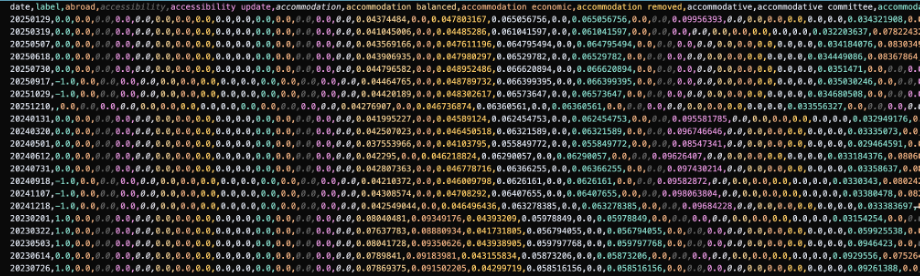
The TF-IDF features are combined with the DFF-based policy labels into a single dataset containing:

• 220 observations
• 1,431 features (unigrams and bigrams)

Limitations

The original plan was to compare models trained on FOMC statements and meeting minutes. However, the meeting minutes are substantially longer, which made data preprocessing and feature construction much more complex than expected. To keep the project manageable, the analysis focuses only on FOMC statements, potentially omitting richer policy discussions.

In addition, the TF-IDF representation with bigrams may not be optimal. Several high-weight phrases (e.g. “assessment account”, “assessment likely”, “committee today”) appear to have limited economic relevance and may introduce noise.

Future Plans

The next step is to introduce a clear train–test split to evaluate out-of-sample predictive performance. Baseline models such as logistic regression and random forest classifiers will be trained and compared. Finally, additional data visualization will be used to improve interpretability and better communicate the relationship between policy language and interest rate decisions.