Predicting Commodity Prices with oLDA (by Group "Market Decoders")

Abstract

Our project aims to explore the relationship between financial news narratives and commodity price fluctuations. Specifically, we utilize Online Latent Dirichlet Allocation (oLDA) to identify latent topics in news streams, quantify the news attention allocated to these topics over time, and use these attention signals to forecast future commodity prices.

First, we built a comprehensive dataset that includes real-time financial news (covering things like commodity market trends, macroeconomic shifts, and policy announcements). During the data preprocessing stage, we standardized the text format, removed irrelevant stuff (like unnecessary metadata and duplicate content), and converted the unstructured news text into a format that works for topic modeling algorithms.

Since we’re still in the middle of model training, there are no visual charts in this blog post for now.

Workflow Overview

(a) Data Collection

To figure out how news affects commodity prices, we needed news data that meets three key needs:

1.Market-relevant: Commodity prices depend on business/economic/policy news, so we stuck to the "business" category (it’s what moves markets).

2.Time-consistent: Prices change daily, so we pulled 2022–2025 news to align with long-term price trends.

3.Enough volume: We needed ~1,100–1,200 articles/month (56,578 total) to spot shifting themes (like "supply shortages" or "rate hikes").

Mediastack News API was perfect here: it lets us filter by category, grab historical data, and scale up easily—so our dataset matches real market news flow.

   # Sample code for fetching news metadata via Mediastack API
   import http.client, urllib.parse, json

   conn = http.client.HTTPConnection('api.mediastack.com')
   params = urllib.parse.urlencode({
      'access_key': 'YOUR_ACCESS_KEY',
      'categories': 'business', 
      'sort': 'popularity',
      'limit': 100
   })

   conn.request('GET', '/v1/news?{}'.format(params))
   res = conn.getresponse()
   data = json.loads(res.read().decode('utf-8'))

Timeframe: 2022 - 2025(We can only get 4-your data from this source,but it is enough for our project)
Volume: Approximately 1,100 to 1,200 articles per month.
Total Dataset: 56,578 articles.

(b) Data Preprocess_1.0

First, we import necessary libraries, load the raw news dataset from an Excel file, and check the basic structure of our data.

   import pandas as pd
   import nltk
   from nltk.corpus import stopwords
   import jieba
   import re
   import json
   import os

   # 1. Load the dataset
   file_path = 'news/news_2025_12_with_content.xlsx'
   df = pd.read_excel(file_path, engine='openpyxl')

   # 2. Data Exploration
   # Display basic information about the dataframe
   print(f"Data length: {len(df)}")
   print(f"Data columns: {len(df.columns)}")
   print("Column names: ", df.columns.tolist())
   # Show the first 5 rows to verify the data
   print(df.head(5))

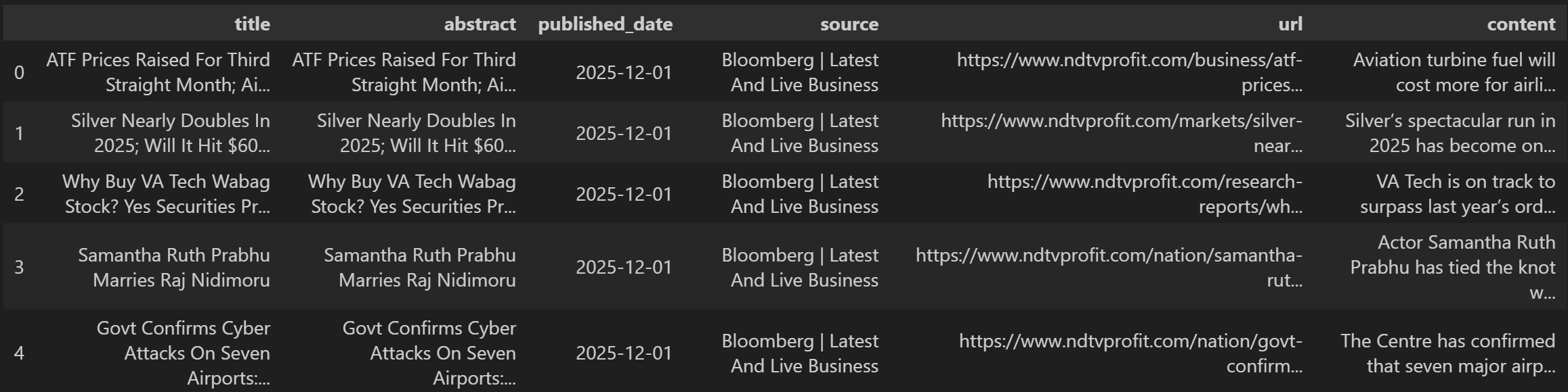
The structure of the dataset is shown in the figure below:

datastructure1

Next, we clean and organize the dataset with three key steps:

1.Data Cleaning: We replace the placeholder text "Failed to retrieve content" in the content column with empty strings to remove invalid entries.

2.Data Transformation: We convert the published_date column to datetime format (to handle time-based grouping later).

3.Date-Based Grouping: We group news entries by their publication date, organizing them into a dictionary where each key is a date (as a string) and the value is a list of daily news details (like title, abstract, and content).

Here’s the code for these steps:

   # Data Cleaning
   # We replace the "Failed to retrieve content" with empty string.
   df.loc[df['content'].str.contains('Failed to retrieve content', case=False, na=False), 'content'] = ''

   # Data Transformation
   # Convert 'published_date' column to datetime objects
   df['published_date'] = pd.to_datetime(df['published_date'], errors='coerce')

   # Grouping Data by Date
   # We organize the news entries into a dictionary
   date_grouped_data = {}
   for date, group in df.groupby('published_date'):
      date_str = str(date)
      daily_list = []

      # Build a list of dictionaries
      for _, row in group.iterrows():
         daily_list.append({
               'title': row['title'],
               'abstract': row['abstract'],
               # Convert timestamp to ISO format string
               'published_date': row['published_date'].isoformat() 
               if pd.notnull(row['published_date']) else None,
               'source': row['source'],
               'URL': row['url'],
               'content': row['content']
         })

      date_grouped_data[date_str] = daily_list

Finally, we save the cleaned and grouped data for later use in topic modeling:

1.Prepare Output Folder: We first create a folder (transformed_data) to store the processed data (if it doesn’t already exist).

2.Save Grouped Data: We export the date-grouped news data (from the previous step) as a JSON-formatted text file (2025_12.txt), using UTF-8 encoding to preserve special characters.

3.Verify Saving: We print the file path and size to confirm the data is saved successfully.

Here’s the code for this step:

   # Save Processed Data
   output_directory = 'transformed_data'
   if not os.path.exists(output_directory):
      os.makedirs(output_directory)

   output_file = os.path.join(output_directory, '2025_12.txt')

   # Save the data as a JSON formatted text file with UTF-8 encoding
   with open(output_file, 'w', encoding='utf-8') as f:
      json.dump(date_grouped_data, f, ensure_ascii=False, indent=2)

   # Final Verification
   print(f"Data saved as {output_file}")
   print(f"File size: {os.path.getsize(output_file) / 1024:.2f} KB")

This is a example of our JSON formatted text data:

   {
   "2025-12-01": [
      {
         "title": "News Title",
         "abstract": "News Abstract",
         "published_date": "2025-12-01T00:00:00",
         "source": "Source Name",
         "URL": "News URL",
         "content": "Cleaned news content"
      }
   ]
   }

(c) Model and Methodology

Our workflow draws inspiration from recent literature in financial text analysis. The core idea is to move beyond simple sentiment analysis to tracking thematic shifts in news.

Topic Modeling (oLDA): We apply oLDA to decompose the high dimensional text data into $K$ latent topics. Unlike static LDA, oLDA adapts to the streaming nature of news.
Quantifying News Attention: For each document $d$ at time $t$, we infer the topic proportion $\theta_d$. We aggregate these to define the News Attention $N_{k,t}$ for topic $k$ at time $t$.
Correlation & Forecasting: We employ sparse regression and multivariate time-series models to isolate robust predictive signals.
- LASSO Regression: We utilize LASSO (Least Absolute Shrinkage and Selection Operator) to handle the high dimensionality of our topic space ($K$ topics). By imposing an $L_1$ penalty, LASSO selects the most relevant topics for forecasting commodity returns while avoiding overfitting.
$$\min_{\beta} \Big( ||r_{t+1} - \mathbf{N}_t\beta||_2^2 + \lambda ||\beta||_1 \Big)$$
- Vector Autoregression (VAR): We implement a VAR model to capture the dynamic interdependencies between news attention and commodity price movements. This allows us to analyze impulse response functions identifying how a sudden spike in a specific narrative (e.g., "Inflation") impacts commodity returns over subsequent periods.

Problems encountered and Solutions

Transitioning from raw text to predictive signals involved overcoming significant hurdles. Below we detail the three major challenges we faced and our technical solutions.

(a) The Abstract Limitation

The Mediastack API efficiently provides metadata, but often restricts content to abstracts or snippets. Relying solely on abstracts fails to capture the rich semantic context required for accurate topic modeling.

Solution: We integrated the newspaper3k Python package. We built a scraper pipeline that iterates through the URLs provided by the API to fetch and parse the full article text, ensuring our model learns from the complete narrative.

   from newspaper import Article

   def get_full_article(url):
      try:
         article = Article(url)
         article.download()
         article.parse()
         return article.text
      except Exception as e:
         return None

(b) Choosing the Right Model: LDA vs. oLDA

Standard Latent Dirichlet Allocation (LDA) assumes that documents are exchangeable, meaning the order of documents does not matter. However, financial news is intrinsically dynamic; the vocabulary and themes evolving in 2022 differ from those in 2025. Standard LDA essentially learns a static topic distribution $\Phi$ over the entire period.

We adopted Online LDA (oLDA) to respect the time-series nature of our data. In oLDA, the model processes data in mini-batches (time windows). The topic-word distribution $\Phi_t$ is updated based on the previous state $\Phi_{t-1}$ and the new batch of documents.

Let $\beta_{k, v}$ represent the weight of term $v$ in topic $k$. In oLDA, we update the variational parameters $\lambda$ based on the gradient from the current mini-batch to approximate the posterior:

$$ \lambda_{t} \leftarrow (1 - \rho_t)\lambda_{t-1} + \rho_t \tilde{\lambda}_t $$

This moving average approach allows the model to "evolve" with the market narratives.

(c) Refining Topic Quality

Our initial oLDA results yielded topics that were incoherent and dominated by noise. A slice of our initial raw output looked like this:

Topic 00: apology, beta, friend, misleading, style...
Topic 01: trump, burst, spikes, upside, naidu...
Topic 07: silver, radar, codes, pro, suggest...

Why was this not expected? The terms were a mix of stop words, irrelevant proper nouns (e.g., "naidu", "chouhan"), and generic verbs that carried no specific economic meaning. This "bag-of-words" noise obscures the underlying economic signal. To fix this, we implemented a three-step enhancement strategy.

(i) Rigorous Preprocessing(Data Preprocess_2.0)

We implemented a strict preprocessing pipeline. We first stripped non-alphabetical characters and lowercased all text to reduce vocabulary size. We then applied a custom rule-based lemmatizer/stemmer designed to normalize derivative words without over-stemming.

The rules are applied in the following order (where $x$ is a candidate term):

"sses" $\to$ "ss": Simplify plural forms ending in double-s.
"ies" $\to$ "y": Normalize plural/variant endings like "stories" to "story".
Trailing "s": Remove standard plurality.
Trailing "ly": Remove adverbial suffixes.
Trailing "ed": Remove past tense markers (replace with "e" if needed for root preservation).
Trailing "ing": Handle continuous tenses. If "ing" follows double consonants, remove "ing" and one consonant; otherwise just remove "ing".
Length Filter: Remove words with fewer than 3 letters to eliminate abbreviations and noise.

This part of the code is quite extensive, the code below is a Code Skeleton of our process.For the complete and rigorous data preprocessing code, please refer to the data_preprocess_word_reconstruct.ipynb file in the GitHub repository of our Project, which includes detailed preprocessing steps with comprehensive comments:

Rigorous Preprocessing Code

# 1. Configuration & Dependency Section
# Define INPUT/OUTPUT directories and initialize cleaning paths.
# Ensure environment readiness before processing starts.

# 2. Rule Loading Module
def load_cleaning_rules():
    """ 
    Scans CLEANING_DIR for CSV (Metadata tags) and TXT (Stopwords) files.
    Aggregates noise-reduction rules into high-speed memory sets.
    """
    pass

# 3. Core NLP Engine (Processing Blocks)
def light_lemmatize_term(word):
    """ 
    Implements light stemming rules (a-f):
    Handling suffix stripping (sses/ies), plural removal, 
    adverb reduction (ly), and silent-e/consonant-doubling (ing).
    """
    pass

def process_field_text(text):
    """ 
    Main cleaning pipeline for text fields:
    Regex cleaning -> Tokenization -> Stemming -> Length Filtering.
    """
    pass

# 4. Noise Reduction & Metadata Filtering
def apply_last_step_noise_reduction(record):
    """ 
    Two-tier filtering strategy:
    1. Term-level: Removes URL remnants and loaded stopwords.
    2. Article-level: Drops records matching CSV 'Bad Tags' (Title/Source).
    """
    pass

# 5. Pipeline Orchestration (Main Execution)
def main():
    """ 
    Iterates through all JSON files in INPUT_DIR.
    Coordinates the pipeline flow and saves non-empty refined datasets.
    """
    pass

if __name__ == "__main__":
    main()

(ii) Rescaling Topic-Term Weights

Standard LDA defines a topic by high-probability words. However, common words (e.g., "market", "price") have high probability across all financial topics, making them poor discriminators.

We rescaled the weights to prioritize words that are specific to a topic relative to the general corpus. Let $\phi_{k,v}$ be the probability of term $v$ in topic $k$ (from LDA components). Let $f_v$ be the marginal probability of term $v$ in the entire corpus.

We calculate the Scaled Weight $\tilde{w}_{k,v}$ as:

$$\tilde{w}_{k,v}=\frac{\phi_{k,v}}{f_v + \epsilon}$$

   # 1. Get Topic-Term distribution (Phi)
   topic_term_counts = lda.components_
   topic_term_distr = topic_term_counts / topic_term_counts.sum(axis=1)[:, np.newaxis] # K x V

   # 2. Get Corpus Term Frequency (f_v)
   corpus_term_counts = np.array(X_all.sum(axis=0)).flatten()
   corpus_term_distr = corpus_term_counts / corpus_term_counts.sum() # 1 x V

   eps = 1e-10

   # 3. Phi_{k,v} / f_v
   scaled_weights = topic_term_distr / (corpus_term_distr[np.newaxis, :] + eps)

$\phi_{k,v}$: The importance of the word in the topic.
$f_v$: The importance of the word generally.

By dividing by $f_v$, we penalize generic words and boost distinctive terms. (e.g., "inflation" might be common, but "hyperinflation" is rare and topic-specific).

(iii) Topic Number Selection

Selecting the optimal number of topics $K$ is crucial. If $K$ is too small, distinct themes (e.g., "Geopolitical Risk" vs. "Monetary Policy") merge. If $K$ is too large, topics become fragmented and unintelligible. We try to iterate through potential values of $K$, balancing model complexity with interpretability.

3. Future Direction

We are currently evaluating the effectiveness of our refined topics.

Topic Quality Assessment: We are quantitatively measuring the coherence and distinctiveness of the topics generated by the oLDA model with the new scaling weights.
Forecasting Model: The next step is to feed these News Attention signals into the regression model defined in section 1(c) to test their predictive power on Commodity Prices.