Abstract
Our project aims to explore the relationship between financial news narratives and commodity price fluctuations. Specifically, we utilize Latent Dirichlet Allocation (LDA) to identify latent topics in news streams, quantify the news attention allocated to these topics over time, and use these attention signals to forecast future commodity prices.
LDA Workflow: From News Text to Temporal Attention Signals
In the previous blog, we discussed the idea of using online topic modeling (oLDA) to capture the temporal evolution of financial news narratives from a methodological perspective. In this post, we focus on the implementation details and describe our topic modeling workflow. In practice, we adopt a Batch LDA approach rather than oLDA, combined with temporal grouping. This design allows us to maintain stable and interpretable topics while constructing news topic attention signals that vary over time.
Step 1: Data Preparation
We organize the cleaned news data into a time-ordered document collection by standardizing publication timestamps, selecting valid text content, and filtering out noisy or low-information articles, which serves as the input for subsequent topic modeling.
   #Sample code for data preparation
   def prepare_articles() -> List[Article]:
    articles = []

    for file_path in sorted(data_path.glob("*.txt")):
        daily_news = json.load(open(file_path, "r", encoding="utf-8"))

        for news_list in daily_news.values():
            for item in news_list:
                if not item.get("published_date"):
                    continue

                published_at = dt.datetime.strptime(
                    item["published_date"], "%Y-%m-%dT%H:%M:%S"
                )

                text = (item.get("content") or item.get("abstract") or "").strip()
                if len(text.split()) < 5:
                    continue

                articles.append(
                    Article(
                        description=text,
                        published_at=published_at,
                    )
                )

    return sorted(articles, key=lambda x: x.published_at)
Step 2: Text Representation
To convert text content into numerical features that can be directly processed by the topic model, we adopt a classic Bag-of-Words representation. We apply basic text normalization, English stopword removal, unigram and bigram features, and document frequency filtering to reduce noise and improve topic quality.
   #Example code for text representation
   vectorizer = CountVectorizer(
       stop_words="english",
       max_df=0.6,
       min_df=5,
       ngram_range=(1, 2),
       max_features=50000,
   )

   texts = [article.text for article in articles]
   X_all = vectorizer.fit_transform(texts)
   vocabulary = np.array(vectorizer.get_feature_names_out())
Step 3: Batch LDA Topic Modeling
After constructing the text features, we train the topic model using Batch LDA on the full news corpus. In our implementation, we set the number of topics to K=100 to balance topic granularity and interpretability. We also apply sparse priors so that each document is associated with only a few topics and each topic is represented by a limited set of keywords, which improves topic focus and supports manual labeling.
   #Example training code
   lda = LatentDirichletAllocation(
       n_components=n_topics,
       learning_method="batch",
       max_iter=20,
       random_state=42,
       doc_topic_prior=0.1,
       topic_word_prior=0.01,
   )

   lda.fit(X_all)
Step 4: Temporal Aggregation
We group news articles by date and construct daily topic attention signals. For each day, we infer topic distributions for all published articles using the trained LDA model and then take their average to obtain a daily topic attention vector. In this way, the static topic modeling results are transformed into dynamic signals suitable for time-series analysis.
   #Example code for temporal aggregation
   daily_attention = {}

   dates = [a.published_at.date() for a in articles]
   article_indices = range(len(articles))

   for date, group in groupby(zip(dates, article_indices), key=lambda x: x[0]):
       indices = [idx for _, idx in group]
       X_slice = X_all[indices]
       doc_topic_distr = lda.transform(X_slice)
   daily_attention[date] = doc_topic_distr.mean(axis=0)
Step 5: Result Export and Analysis
Finally, we extract representative keywords for each topic from the LDA model to support manual topic labeling and economic interpretation. We also export the daily topic attention signals in matrix form so that they can be directly used as input features in subsequent regression or time-series modeling frameworks.
   #Example code for result export
   topic_term_counts = lda.components_
   topic_term_distr = topic_term_counts / topic_term_counts.sum(axis=1)[:, np.newaxis]

   topic_terms = []
   for k in range(n_topics):
       top_indices = topic_term_distr[k].argsort()[::-1][:10]
       top_words = vocabulary[top_indices]
   topic_terms.append(top_words.tolist())
   export_topic_terms(topic_terms, topic_terms_path)
   export_daily_attention(daily_attention, topic_attention_path)
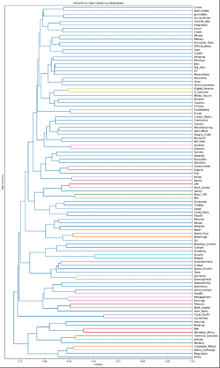
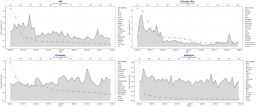
Since the model learns a total of K=100 topics, we select a small number of representative results for visualization based on their semantic content and temporal patterns. The following figures present a subset of the results.
Regression Analysis
Based on topic attentions we obtained above, we did Lasso Regression to do the feature selection and then Multiple Regression to do the validation.
Our model logic flow shows as follows:
1.Input Data: Our input data involves all topic attention scores (θₖ,ₜ) generated by LDA model.
2.Lasso Regression (Feature Selection): We use L1 penalty to shrink irrelevant topics to 0, retaining top 5-8 core topics (e.g., Geopolitics, Supply). The formular we used is shown below:
3.Multiple Regression (Validation): We incorporate selected topics with traditional controls (USD Index, PMI) to test incremental value.
4.Output Result: We quantified coefficients (βₖ) for core topics and verification of ΔR².
Here’s the code for the core regression part:
   # Lasso Five-Factor Selection Algorithm (corresponds to Section III.A of the paper)
   def lasso_selection_fixed_5(X, y, topic_names):
      """
      Find alpha using bisection method such that Lasso retains exactly 5 non-zero variables.
      Then uses Post-Lasso OLS to estimate statistics (p-val, SE, CI).
      """
      # Standardization - corresponds to the procedure on page 3121 of the paper
      scaler_x = StandardScaler()
      scaler_y = StandardScaler()
      X_std = scaler_x.fit_transform(X)
      y_std = scaler_y.fit_transform(y.values.reshape(-1, 1)).flatten()
      low, high = 0.000001, 1.0
      best_alpha = 0.1
      # Iterate to find the appropriate alpha penalty parameter
      for _ in range(30):
         mid = (low + high) / 2
         model = Lasso(alpha=mid, random_state=42, max_iter=10000)
         model.fit(X_std, y_std)
         non_zero_count = np.count_nonzero(model.coef_)

            if non_zero_count == 5:
            best_alpha = mid
            break
            elif non_zero_count > 5:
               low = mid
            else:
               high = mid
      # Re-run the model using the optimal alpha found
      final_model = Lasso(alpha=best_alpha, random_state=42)
      final_model.fit(X_std, y_std)
      # Identify non-zero coefficients
      selected_mask = final_model.coef_ != 0
      selected_indices = np.where(selected_mask)[0]
      if len(selected_indices) == 0:
         return pd.DataFrame(), 0.0
      # --- Post-Lasso OLS for Inference ---
      # Select the features identified by Lasso
      X_selected = X_std[:, selected_indices]
      # Add constant for OLS (intercept)
      X_selected_const = sm.add_constant(X_selected)
      # Fit OLS
      ols_model = sm.OLS(y_std, X_selected_const).fit()
      results = []
      # Loop through selected indices
      # Note: OLS params has intercept at index 0, so features are at i+1
      for i, idx in enumerate(selected_indices):
         topic = topic_names[idx]
         # OLS Stats
         coef = ols_model.params[i+1]
         std_err = ols_model.bse[i+1]
         p_val = ols_model.pvalues[i+1]
         conf_int = ols_model.conf_int()[i+1]
         results.append({
            'Topic': topic,
            'Coefficient': coef,
            'Std_Err': std_err,
            'P_Value': p_val,
            'CI_Lower': conf_int[0],
            'CI_Upper': conf_int[1]
         })
      selected_df = pd.DataFrame(results)
      selected_df = selected_df.sort_values(by='Coefficient', ascending=False)
      # Use OLS R-squared for the explanatory power of the selected factor model
      r2 = ols_model.rsquared
      return selected_df, r2
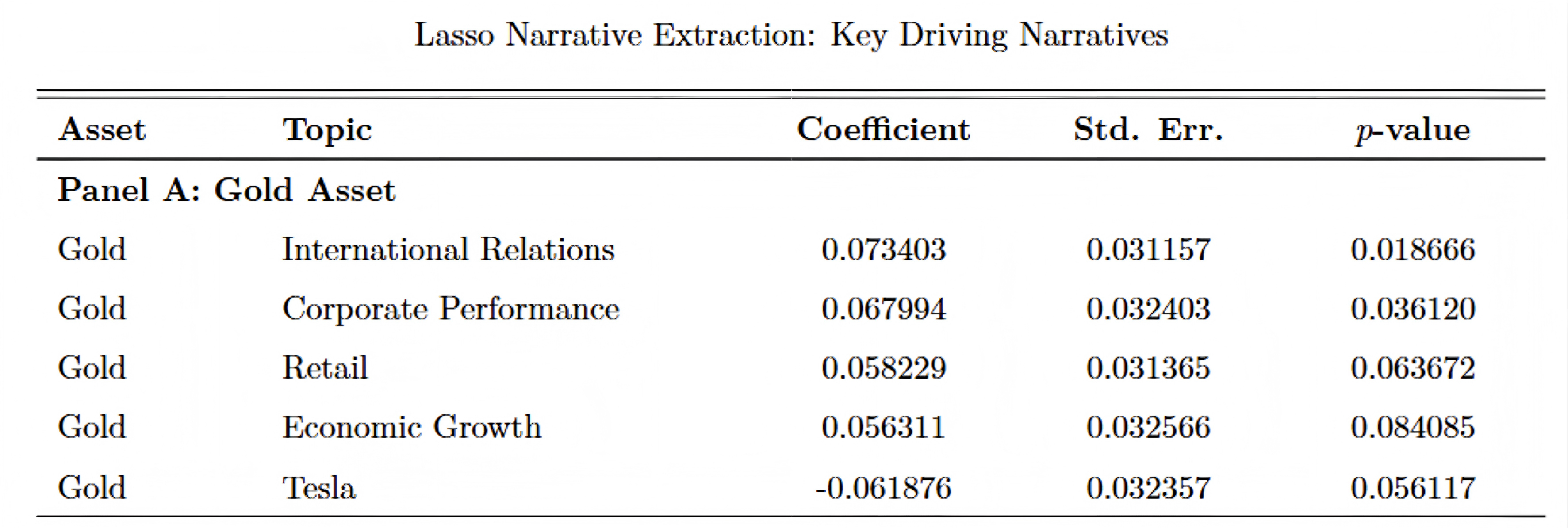
As the output for our lasso regression, we can see from the table that International Relations and Corporate Performance carry significantly positive correlations (e.x. 1% increase in attention to international relations raises prices by about 0.07%), which indicates that gold benefits from macro political uncertainty
Prediction based VAR
Further to make our analysis more practical for guiding trading strategies, we use VAR model to predict future gold returns. Except for the topic attentions we created, we also add macroeconomic variables into the model, which can be seen in the formular below:
,where model:
Specifically, we utilized 80% of the data for training and the remaining 20% for testing. The model's performance was evaluated using key metrics: the Mean Squared Error (MSE) was 0.0243%, and the Mean Absolute Error (MAE) was 1.1313%. These metrics indicate that our model is highly effective in capturing the dynamics of gold returns, providing a reliable approach for short-term market forecasting.
As the outcome of our analysis, in the graph below, the blue line represents the actual gold return data, while the red dashed line indicates the model's rolling forecast.
.png)
Problems encountered and Solutions
Transitioning from raw text to predictive signals involved overcoming significant hurdles. Below we detail the three major challenges we faced and our technical solutions.
(a) Choosing the Right Model: LDA vs. oLDA
Standard Latent Dirichlet Allocation (LDA) assumes that documents are exchangeable, meaning the order of documents does not matter. However, financial news is intrinsically dynamic; the vocabulary and themes evolving in 2022 differ from those in 2025. Standard LDA essentially learns a static topic distribution \(\Phi\) over the entire period.
Online LDA (oLDA) to respect the time-series nature of our data. In oLDA, the model processes data in mini-batches (time windows). The topic-word distribution \(\Phi_t\) is updated based on the previous state \(\Phi_{t-1}\) and the new batch of documents.
However, while theoretically appealing for time-series data, the practical implementation yielded suboptimal results. The topics generated exhibited low semantic coherence, with each topic's top keywords often spanning multiple unrelated domains rather than converging into a single interpretable theme.
A slice of our initial raw output looked like this:
- Topic 00: apology, beta, friend, misleading, style...
- Topic 01: trump, burst, spikes, upside, naidu...
- Topic 07: silver, radar, codes, pro, suggest...
Given the challenge with the Online LDA (oLDA), we revisited the Standard Latent Dirichlet Allocation (LDA) but introduced several targeted enhancements to address its limitations while preserving topic quality. The key modifications involved both Feature Engineering, Model Configuration and Topic Choice:
1.Feature Engineering : We incorporate Bigrams into our text processing pipeline to capture meaningful multi-word expressions that frequently appear in financial discourse. By extending beyond individual words to include two-word combinations, we can better represent compound financial terms that carry specific semantic meaning distinct from their constituent parts.
For instance, the phrase "interest_rate" functions as a cohesive financial concept that differs significantly from analyzing "interest" and "rate" separately; similarly, "federal_reserve," "central_bank" and "stock_market" represent institutional and market entities whose meanings would be diluted if broken into individual components.
Here’s the code for this step:
   # Extract the raw text content from all Article objects
   texts = [article.text for article in articles]

   # Initialize CountVectorizer for converting text documents to a matrix of token counts
   vectorizer = CountVectorizer(
      stop_words="english",   # Remove common English stop words (the, and, is, etc.)
      max_df=0.6,             # Ignore terms that appear in more than 60% of documents
      min_df=5,               # Ignore terms that appear in fewer than 5 documents
      ngram_range=(1, 2),     # Include both single words (unigrams) and word pairs (bigrams)
      max_features=50000,     # Limit to top 50,000 features by frequency to control memory usage
   )
   # Transform the text collection to a document-term matrix
   X_all = vectorizer.fit_transform(texts)

   # Get the feature names (vocabulary) as a numpy array
   vocabulary = np.array(vectorizer.get_feature_names_out())
2.Model Configuration :
2.1 We configure the doc_topic_prior (\(\alpha\)) and topic_word_prior (\(\beta\)) hyperparameters with intentionally sparse values to align with the inherent structure of financial discourse.
The doc_topic_prior of 0.1 encodes our assumption that financial news articles typically concentrate on a limited number of thematic domains, encouraging each document to associate strongly with only one or two primary topics rather than distributing its attention uniformly across all possibilities. This reflects the practical reality that a news piece about "central bank policy decisions" primarily belongs to monetary policy discussions, with only peripheral connections to other financial themes.
The topic_word_prior of 0.01 implements our expectation that meaningful financial topics should be characterized by a focused set of terminology, promoting each topic to be defined by a coherent cluster of semantically related terms rather than a diffuse collection of unrelated vocabulary.
This dual sparsity constraint produces more interpretable and actionable topic structures where both documents and topics exhibit clear thematic identities, which proves particularly valuable for financial analysis where precise categorization and clear conceptual boundaries enhance downstream applications like sentiment tracking and thematic trend analysis.
Here’s the code for this step:
   # LDA model configuration for financial text analysis
   lda = LatentDirichletAllocation(
      n_components=n_topics,        # Topic count
      learning_method="batch",      # Train once on all data
      max_iter=20,                  # Ensure convergence
      random_state=42,              # Reproducible results
      doc_topic_prior=0.1,          # Documents focus on few topics
      topic_word_prior=0.01,        # Topics focus on few key words
)
2.2 We fundamentally replace the incremental partial_fit approach (lda.partial_fit(X_slice)) with a comprehensive single-pass fit operation on the entire document collection.
This paradigm shift prioritizes thematic stability over temporal adaptability, establishing a fixed set of topic definitions that remain semantically constant throughout our analysis timeframe. By training the model once on the complete corpus, we obtain a consistent reference framework where each topic retains its conceptual identity across all time periods, enabling reliable longitudinal comparison of topic prevalence and eliminating the interpretive ambiguity introduced by evolving topic compositions. This methodological choice recognizes that for financial news analysis, the ability to track how attention to well-defined thematic areas fluctuates over time outweighs the theoretical benefit of modeling gradual conceptual evolution.
Here’s the code for this step:
   for date, indices in date_groups:
    X_slice = X_all[indices]                      # Get documents for this date
    doc_topic_distr = lda.transform(X_slice)      # Get topic distributions
    avg_attention = doc_topic_distr.mean(axis=0)  # Average across articles
    daily_attention[date] = avg_attention         # Store daily topic attention
3.Topic Choice : We select topic keywords based directly on their \(\phi\) probabilities (the conditional probability P(word|topic)) rather than using lift scores that scale these probabilities by corpus-wide term frequencies. This methodological choice prioritizes term relevance within topics over statistical distinctiveness, ensuring that each topic's most characteristic words are those that appear most frequently when the topic is expressed, regardless of their overall prevalence in the financial discourse.
By focusing on high-probability terms, we obtain more semantically coherent and interpretable topic descriptors that better align with recognizable financial concepts, which proves essential for downstream analytical tasks where clear topic identification directly supports investment decision-making and market narrative analysis.
Here’s the code for this step:
   # Topic-term count matrix from trained LDA
   topic_term_counts = lda.components_
   # Convert to probability distribution φ
   topic_term_distr = topic_term_counts / topic_term_counts.sum(axis=1)[:, np.newaxis]

   topic_terms = []
   for k in range(n_topics):
      top_indices = topic_term_distr[k].argsort()[::-1][:10]  # Sort terms by φ probability for topic k
      top_words = vocabulary[top_indices]                     # Get actual words from vocabulary array
      topic_terms.append(top_words.tolist())                  # Store as list for this topic
(b) The Modification of the VAR Model
- Problem: In the initial VAR(1) forecasting results, the predicted gold returns appear excessively smooth and close to zero, forming an almost flat line in the forecast horizon. This phenomenon arises because the standard VAR forecast reports the conditional mean forecast, which assumes that future shocks are zero. Since financial return series, including gold returns, are typically close to mean zero and exhibit weak persistence, the conditional expectation naturally converges quickly to its long-run mean. As a result, although the model is statistically well specified, the deterministic VAR forecast fails to reflect the volatility and uncertainty that characterize real-world financial markets.
.jpg)
- Solution: To address this limitation, we adopt an alternative forecasting approach based on stochastic simulation of the VAR model. Instead of setting future innovations to zero, this method repeatedly draws random shocks from the estimated residual distribution and propagates them through the VAR dynamics. By explicitly incorporating these random shocks, the simulated forecasts capture both the conditional mean dynamics and the inherent uncertainty of the system. Consequently, the resulting forecast paths exhibit realistic fluctuations and volatility, producing predictions that more closely resemble observed market behavior. This approach does not alter the underlying VAR structure; rather, it provides a more informative representation of potential future outcomes by moving from a deterministic forecast to a probabilistic, simulation-based forecast framework.
Here's the code for the solution:
   import pandas as pd
   from statsmodels.tsa.api import VAR
   import matplotlib.pyplot as plt

   df = pd.read_stata("data_dropna.dta")
   df['date'] = pd.to_datetime(df['date'])
   df = df.set_index('date')
   cols = ['gold_ret', 'topic7', 'dvix', 'ddxy']
   df_var = df[cols].dropna()
   model = VAR(df_var)
   results = model.fit(1)
   sim = results.simulate_var(
      steps=30,
      seed=42
   )
   sim_df = pd.DataFrame(
      sim,
      columns=df_var.columns,
      index=pd.date_range(df_var.index[-1], periods=31, freq='B')[1:]
   )
   plt.figure(figsize=(10,5))
   plt.plot(df_var['gold_ret'].iloc[-200:], label='Actual', color='black')
   plt.plot(sim_df['gold_ret'], label='Forecast', color='blue')
   plt.legend()
   plt.title("Simulated VAR(1) Forecast of Gold Returns")
   plt.show()
The simulated forecast result below introduces random shocks and illustrates one possible future path rather than the conditional mean forecast.
.png)
Conclusion
In conclusion, this project demonstrates the predictive power of unstructured financial news in forecasting commodity markets. By transforming textual information into quantitative signals using LDA and validating them through Lasso and VAR frameworks, we uncovered significant correlations between topic attention and price movements. While we focused exclusively on limit metal forcast due to time constraints, our methodology provides a robust foundation for analyzing commodity and even broader asset classes, highlighting the immense value of NLP in modern financial decoders.