By Group "Lighthouse Securities"
Lighthouse Securities: The trusted light for your financial journey
1. Introduction
Welcome back to our series on central bank communications and market dynamics. In our previous blogpost, we laid the groundwork for our project, exploring the ideation process and the technical hurdles of scraping high-quality textual data from both the Federal Reserve (FED) and the European Central Bank (ECB). We also established our data sources for market volatility across the US and European markets.
With the raw data safely in our hands, we move from collection to the core of our technical pipeline. In this post, we will dive into the nuances of data cleaning, structuring, and the initial natural language processing (NLP) techniques we are employing to turn dense policy accounts into quantifiable financial sentiment.
2. Data Cleaning and Structuring
When we first moved from data collection to data cleaning, we assumed this would be a relatively mechanical step — removing HTML tags, fixing encoding issues, and preparing the text for NLP models.In practice, this stage turned out to be one of the most time-consuming and conceptually challenging parts of the entire project.
The main difficulty was not technical, but institutional. FOMC and ECB minutes differ not only in length, but also in structure, writing style, and—most importantly—timing.
A mistake we initially made was to align market data directly with the release dates of the minutes. This created a subtle form of look-ahead bias, as the market often reacts to the underlying meeting information before the official publication.
Below is a simplified version of the cleaning logic we eventually settled on: In hindsight, this stage taught us that in text-based financial research, data cleaning is not a preprocessing step, but an economic modeling decision.
# Core cleaning stages
text = remove_html_tags(text)
text = fix_encoding(text)  # NFKC normalization
text = remove_names_and_titles(text)  # Powell, Lagarde, etc.
text = extract_substantive_content(text)  # Skip attendance sections
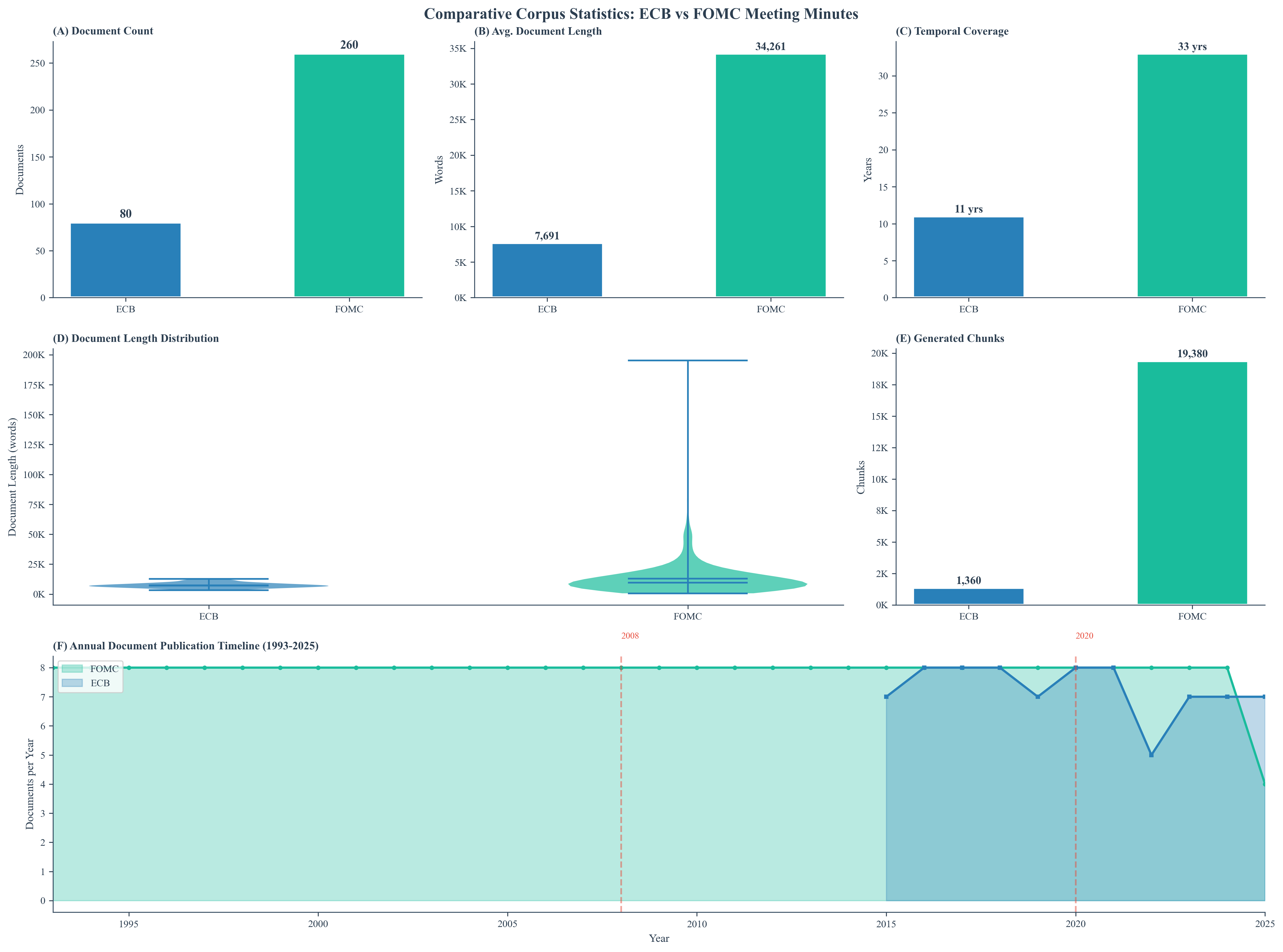
After deduplication, we retained 340 documents (ECB: 80, FOMC: 260) spanning 33 years. The two corpora differ significantly—FOMC minutes average 34,261 words versus ECB's 7,691 words.
3. Natural Language Processing Techniques
3.1 Cosine Similarity
The first thing we needed to do in both Approach 1 and Approach 3 was the embedding of the minutes. So we looked for models that could provide us with high-quality embeddings for our text data.
And we found BERT-based models are quite popular in the academic community for various NLP tasks, including text classification and sentiment analysis. But the limits of BERT actually pushed us to explore more advanced models like Qwen3-Embedding-8B, which has less limitations on the input text length and can handle longer documents more effectively.
But when we actually started to try to run the model on the Kaggle platform, we found that the model was quite resource-intensive and required a lot of computational power to run efficiently. So we had to turn to OpenRouter, which provided us with an API to access the Qwen3-Embedding model without needing to run it locally.
from openai import OpenAI

client = OpenAI(
    base_url=OPENROUTER_BASE_URL,
    api_key=API_KEY,
)

def embedding_with_usage(text: str, model_name="qwen/qwen3-embedding-8b"):
    embedding = client.embeddings.create(
        extra_headers={
            "HTTP-Referer": "https://github.com/Lighthouse-Securities/FOMC-Analysis",
            "X-Title": "Central Bank Analysis",
        },
        model=model_name,
        input=text,
        encoding_format="float",
        extra_body={
            "usage": {
                "include": True
            }
        }
    )

    try:
        print("Input tokens:", embedding.usage.prompt_tokens)
        print("Total tokens:", embedding.usage.total_tokens)
        print("Cost:", embedding.usage.cost, "credits")

        return embedding.data[0].embedding
    except AttributeError:
        print(embedding.model_extra['error']['message'])
        return None
Then we used the Qwen3-Embedding model to generate embeddings for each of the FOMC and ECB minutes. During the embedding, we found that even though the model could handle longer texts, some of the minutes were still too long to fit into a single input. So we had to truncate some of the minutes to fit within the model's input limits.
for date, text in minutes.items():
    ...
    text = text[:128000]
    ...
3.2 LLM Classification
When setting out on our analysis using Large Language Models (LLMs), we were planning to use state-of-the-art (SOTA) models for the best results. However, we quickly encountered a significant hurdle; being based in Hong Kong. Access to leading models from OpenAI, Google (Gemini Flash 3.0 was our original choice), and Anthropic was restricted due to regulatory constraints. This limitation forced us to pivot our approach and explore alternative models available through OpenRouter.
We aimed to keep costs low while still achieving reliable performance, so we looked for the best freely accessible model on OpenRouter. After evaluating several options, we settled on Xiaomi's Mimo v2 Flash model. While not as advanced as some of the restricted models, Mimo v2 Flash provided a good balance between accessibility and performance for our sentiment analysis tasks. The models are easy to use with only a few lines of code:
from openai import OpenAI

client = OpenAI(
    base_url=OPENROUTER_BASE_URL,
    api_key=API_KEY,
)

response = client.chat.completions.create(
    model=model_name,
    messages=[
        {"role": "user", "content": prompt}
    ],
    temperature=0.1
)
We chose a temperature of 0.1 to ensure more deterministic outputs, which is crucial for consistent sentiment scoring. In our testing, the results are still not fully deterministic, but the variance is minimal enough to not significantly impact our regression analyses. After running the LLM classification on both FOMC and ECB minutes, we extracted key features such as sentiment, hawkishness, and inflation concern. These features were then integrated into our regression models to assess their impact on market volatility.
Creating a correct and, ideally, significant regression model is always challenging. We go through many iterations of finding the correct control variables, assessing multicollinearity, handling heteroscedasticity, and other statistical pitfalls. In our analysis, both GDP and CPI had to be dropped due to multicollinearity issues (both for FED and ECB). To deal with heteroscedasticity (tested through a Breusch-Pagan and White test), we used robust standard errors (HC3) throughout our regression analyses.
3.3 Neural Embeddings
In our approach 3, we have two models. The first model, which we called it the baseline model, is quite simple. We just feed the text vectors to feed forward neural network with two hidden layers. On the top of this baseline model, we would like to add some market variables as input, for example the FFR, GDP etc., since an intuitive thinking is that those market variables would also have great influence on the following stock market volitility. But here comes the question: what is a good way to combine the text vectors and market variables? A simple method is that we could concatenate the market variables after the text vecters directly, by which we create a new vector and feed to the FFN. The structure of this simple model is as follow:
import torch
import torch.nn as nn
class easy_fusion_FNN(nn.Module):
    def __init__(self, text_dim, market_dim, fusion_text_dim=128, fusion_mkt_dim=8, combine_dims=[128,8], output_num=1,drop_out=0.3):
        '''
            text_dim: the dimensions of text;
            markrt_dim: the dimensions of the market variables;
            fusion_text_dim: the numble of neurons in the hidden layer in the sub NN for text;
            fusion_mkt_dim: the numble of neurons in the hidden layer in the sub NN for market  variables;
            combine_dims: the number of neurons in combine layer;
            out_num: the number of output layer, since we are doing binary classification, here the out_put=1 defaulty;
            drop_out: value of the dropout() attribute;
        '''
        super(easy_fusion_FNN, self).__init__()

        combine_fusion_dim = text_dim+market_dim
        self.fusion_net = nn.Sequential(
            nn.Linear(combine_fusion_dim, combine_dims[0]),
            nn.ReLU(),
            nn.Dropout(drop_out),
            nn.Linear(combine_dims[0], combine_dims[1]),
            nn.ReLU(),
            nn.Dropout(drop_out),
            nn.Linear(8, output_num)
        )


    def forward(self, text , mkt):
        combined = torch.cat((text, mkt), dim=1)
        return self.fusion_net(combined)
Theoretically speaking, the disadvantage of this model is that text vectors and market data are directly mixed, and the model may struggle to distinguish between two different types of data and may not adequately learn the characteristics of both data. So, we made some adjustments to the model and created a new model, which we called fusion model. The key is that we first used two sub-neural networks to process the text vectors and market variables respectively. Then, we concatenated the outputs of the two sub-networks as the input for the next hidden layer. In this way, the two sub-networks can respectively learn the text features and market features. But the weakness is that the complexity of the model is much more higher which may makes model doen't fit well to our experiment due to the less amount of data. The structure is as follow:
class fusion_FNN(nn.Module):
    def __init__(self, text_dim, market_dim, fusion_text_dim=128, fusion_mkt_dim=8, combine_dims=8, output_num=1,drop_out=0.3):
        '''
            text_dim: the dimensions of text;
            markrt_dim: the dimensions of the market variables;
            fusion_text_dim: the numble of neurons in the hidden layer in the sub NN for text;
            fusion_mkt_dim: the numble of neurons in the hidden layer in the sub NN for market  variables;
            combine_dims: the number of neurons in combine layer;
            out_num: the number of output layer, since we are doing binary classification, here the out_put=1 defaulty;
            drop_out: value of the dropout() attribute;
        '''
        super(fusion_FNN, self).__init__()

        self.text_net = nn.Sequential(
            nn.Linear(text_dim, fusion_text_dim),
            nn.ReLU(),
            nn.Dropout(drop_out),
        )

        self.market_net = nn.Sequential(
            nn.Linear(market_dim, fusion_mkt_dim),
            nn.ReLU(),
            nn.Dropout(drop_out),
        )

        combine_fusion_dim = fusion_mkt_dim + fusion_text_dim
        self.fusion_net = nn.Sequential(
            nn.Linear(combine_fusion_dim, combine_dims),
            nn.ReLU(),
            nn.Dropout(drop_out),
            nn.Linear(8, output_num)
        )


    def forward(self, text , mkt):
        subNN_text = self.text_net(text)
        subNN_mkt = self.market_net(mkt)
        combined = torch.cat((subNN_text, subNN_mkt), dim=1)
        return self.fusion_net(combined)
So, What is the actually performance of the two models? In order to get a more robust result, we trained 1000 separate models using different structures independently, and then tested them on the test set. We took the average of the results from these 1000 tests. The result is quite surprising. In fact, the easy structure works better in our cases.

4. VIX Trading Strategy
Translating textual similarity into a trading signal was not an obvious next step. At first, we were skeptical whether cosine similarity—an abstract NLP metric—could carry any economically meaningful information for a volatility instrument like VIX. The initial thresholds were admittedly heuristic, chosen based on exploratory analysis rather than theory.
if similarity < 0.83:
    signal = 1   # Long VIX
elif similarity > 0.96:
    signal = -1  # Short VIX
Given how easy it is to overfit a low-frequency strategy with few trades, we deliberately focused less on the maximum Sharpe ratio and more on whether performance was stable across neighboring parameters.The presence of a parameter plateau was more important to us than the single best point, as it reduced the risk that our results were driven by accidental parameter tuning.
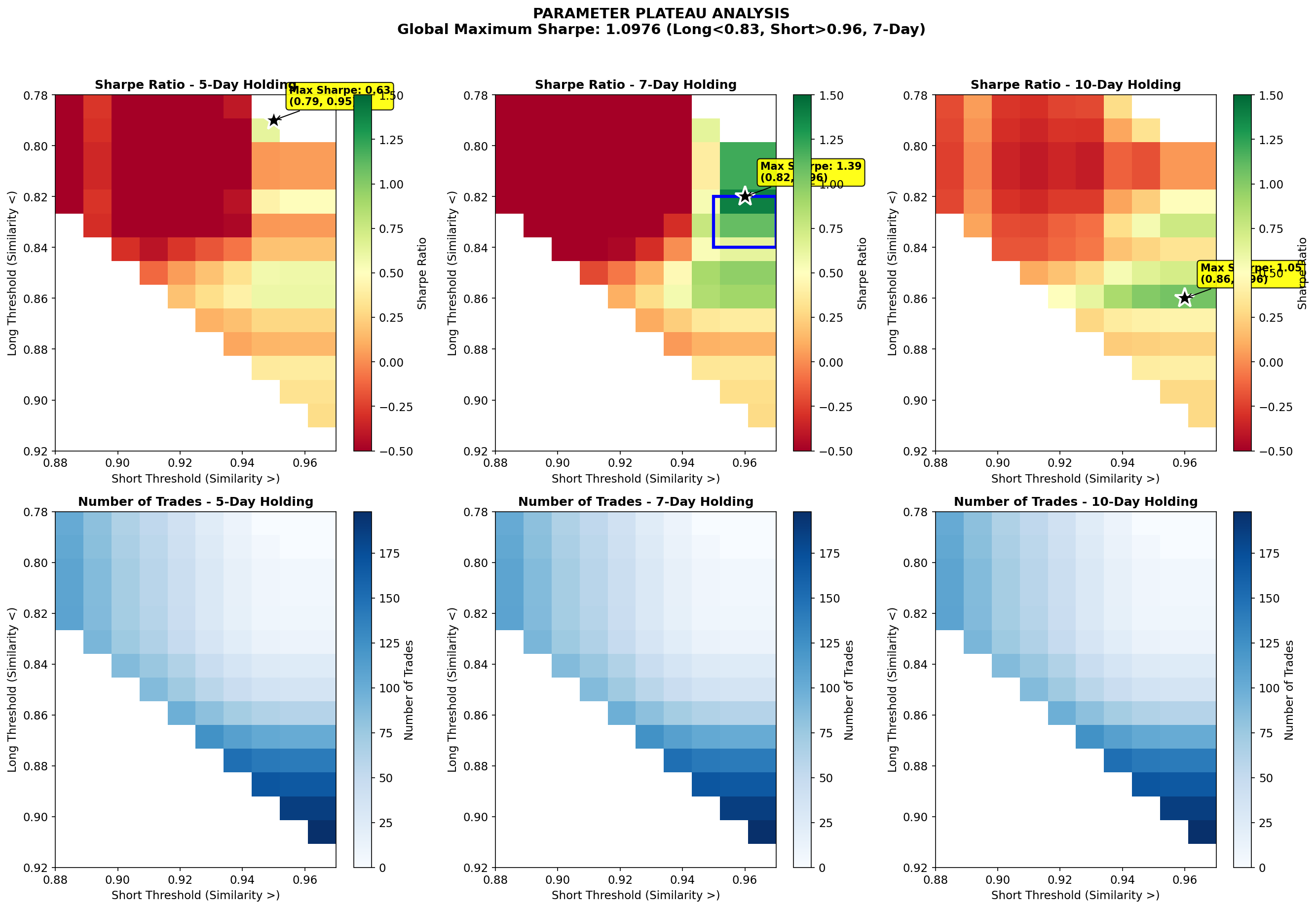
That said, the strategy trades infrequently and is heavily dependent on extreme similarity events. This makes it vulnerable to regime changes and limits its standalone applicability.