Building a robust portfolio optimization framework requires high-quality, multi-dimensional data and a well-structured training environment. This blog walks through our team’s end-to-end workflow, covering data collection from dual sources, preprocessing, and the construction of a reinforcement learning (RL) environment to power portfolio decisions.

Part 1: Data Collection from Stocktwits – Advanced Scraping & Sentiment Analysis

To capture market sentiment and discussions spanning over a decade, we targeted Stocktwits data for 6 core assets from 2012 to 2024. This process required overcoming sophisticated anti-bot measures and navigating unique pagination challenges, followed by sentiment visualization.

1 Advanced Web Scraping & TLS Impersonation

The primary goal was to harvest data for 6 core assets spanning from 2012 to 2024. However, the first hurdle was bypassing the platform's sophisticated bot detection.

Challenge: Defeating TLS Fingerprinting

Standard Python libraries like requests were immediately flagged by Cloudflare (403 Forbidden).

The Solution: curl_cffi for TLS Impersonation

I used the curl_cffi library. Unlike standard requests, curl_cffi allows for impersonation of a real browser's TLS handshake, which is essential for passing modern anti-bot checks.

The Cookie "Clean" Trick

I also implemented a clean_val function to strip non-ASCII characters from raw browser cookies, ensuring the headers remained valid for the HTTP request.

from curl_cffi import requests

def clean_val(v):
    return "".join(i for i in str(v) if ord(i) < 128)

headers = {
    "user-agent": "Mozilla/5.0 (Macintosh; Intel Mac OS X 10_15_7)...",
    "cookie": clean_val(raw_cookie)
}

r = requests.get(url, params={"max": current_max_id}, headers=headers, impersonate="chrome110", timeout=30)

2 Solving the "Temporal Navigation" Problem

Stocktwits uses an ID-based pagination (max_id). Since the platform doesn't allow direct date-based searching, locating data from 2012 among billions of posts required an intelligent search algorithm.

Challenge: The Pagination Abyss

If you jump back too far, you skip data. If you jump too little, the script takes weeks to finish. Furthermore, the API often gets "stuck" returning the same page (Oscillation).

The Solution: Dynamic Jumping & Stuck Detection

Dynamic Leap: My script calculates the distance between the current data's timestamp and the target date. For years after 2020 (high-volume era), it jumps by 3.4 million IDs per month. For earlier, quieter years, it scales down to 1 million IDs.

Oscillation Detection: I added a stuck_count tracker. If the script detects it is receiving the same top_id multiple times, it forces a larger "emergency jump" to break the loop.

if ts.year > year:
    m_diff = (ts.year - year) * 12 + (ts.month - month)
    # Post-2020 data is much denser
    jump = 3400000 * m_diff if ts.year > 2020 else 1000000 * m_diff
    current_max_id -= max(jump, 100000)

if stuck_count >= 4:
    current_max_id -= 2500000
    print(f"Detected oscillation, forcing jump to {current_max_id}")

3 Data Cleaning: Handling Tags

StockTwits text data contains numerous financial asset tags. Some data entries consist almost entirely of tags without substantial content. Initially, we considered removing all tag labels. However, since tags may contribute to the meaning of a sentence, directly deleting them could alter the original semantics. Therefore, we used regular expressions to identify tags and calculated their ratio to the total word count in the text. Data entries with excessively high tag ratios were filtered out.

def calculate_tag_ratio(self, text):
    if pd.isna(text):
        return 0

    text_str = str(text)
    words = text_str.split()

    if len(words) == 0:
        return 0

    tag_count = 0
    for word in words:
        if re.match(self.config['tag_pattern'], word):
            tag_count += 1

    tag_ratio = tag_count / len(words)
    return tag_ratio

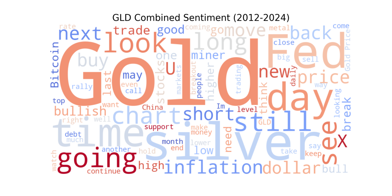
4 Visualization & Sentiment Portraits

I merged the historical datasets for all six assets to generate a visual sentiment profile for the 2012–2024 period. I applied a consistent set of STOPWORDS and cleaning rules across all assets to ensure a fair comparison. This included removing common web noise (http, https, amp, rt) and generic platform terms.

Observation: Asset-Specific Noise Levels

A key finding during the visualization phase was the difference in data quality between assets:

• Specialized Assets ($GLD, $USO): Sentiment was relatively focused on asset-specific trends.

• Market Indices ($SPX): The $SPX data displayed significantly higher noise levels, containing a larger volume of retail "hype" and generic market tags compared to the commodity-linked assets.

my_stopwords = set(STOPWORDS)
my_stopwords.update(['http', 'https', 'amp', 'rt', 'now', 'today', 'stock', 'market', 'will', 'year', 'week'])

wc = WordCloud(
    width=1000, height=500, 
    background_color='white',
    stopwords=my_stopwords,
    max_words=100, 
    colormap='coolwarm'
).generate(full_text)

Part 2: Supplemental News Data Collection with GDELT

To complement Stocktwits sentiment data, we leveraged GDELT (Global Database of Events, Language, and Tone) to automate the download of structured historical news data. This dual-source approach enriched our dataset with broader market narratives.

1 Asset Configuration

We collected news data for six core categories of financial assets:

• Stock Indices: S&P 500 (GSPC), NASDAQ Composite (IXIC), Dow Jones Industrial Average (DJI)

• Commodities: Gold (GOLD), Silver (SILVER), Crude Oil (OIL)

Each asset configuration includes:

{
    "name": "S&P 500 Index",
    "keywords": ["SP500", "SPX", "Standard Poors 500", "S and P 500"],
    "ticker": "$SPX",  # StockTwits format code
    "type": "E"  # Asset type identifier
}

2 System Architecture Design

• Time Range: January 2017 to December 2024

• Granularity Control: Monthly downloads with a maximum of 20 records per month

• Intelligent Date Processing: Automatic calculation of start and end dates for each month

class FinancialAssetsDownloader:
    def __init__(self):
        self.assets_config = {...}
        self.start_year = 2017
        self.end_year = 2024
        self.max_records_per_month = 20

Monthly Data Download Process

The workflow follows a structured cycle: Iterate through each month from 2017 to 2024 → Call GDELT API to retrieve news data → Add asset metadata (asset ID, name, type, etc.) → Save monthly CSV files → Consolidate all monthly data

def download_asset_data(self, asset_id, asset_config):
    asset_name = asset_config["name"]
    keywords = asset_config["keywords"]

    all_data = []

    for year in range(self.start_year, self.end_year + 1):
        for month in range(1, 13):            
            try:
                start_date, end_date = self.get_month_date_range(year, month)

                f = Filters(
                    start_date=start_date,
                    end_date=end_date,
                    num_records=self.max_records_per_month,
                    keyword=keywords,
                    language="English"
                )

                articles_df = self.gd.article_search(f)
                ...
                all_data.append(articles_df)

                month_csv = os.path.join(asset_dir, f"{asset_id}_{year}_{month:02d}.csv")
                articles_df.to_csv(month_csv, index=False, encoding="utf-8-sig")
                ...
            time.sleep(random.uniform(self.min_delay, self.max_delay))
    ...

3 Key Technical Implementations

3.1 Anti-Scraping Strategy

To ensure stable and sustainable access to the GDELT API while respecting server resources, we implemented a comprehensive anti-scraping strategy featuring intelligent delay mechanisms.

# Random delay settings
self.min_delay = 2.0
self.max_delay = 4.0

# Longer delay between assets
delay_time = random.uniform(8, 15)

Technical Rationale:

a. Rate Limiting Compliance:

The random delay between monthly requests (2-4 seconds) prevents rapid-fire queries that could trigger GDELT's rate limiting mechanisms or be mistaken for denial-of-service attacks.

b. Behavioral Mimicry:

By varying the delay times randomly, our system mimics human browsing patterns rather than exhibiting the predictable, machine-like timing of simple automated scripts.

c. Resource Protection:

The longer delays between assets (8-15 seconds) provide breathing room for both our system and GDELT's servers, particularly important when downloading multiple years of data across multiple assets.

3.2 GDELT API Integration

The core of our data collection system leverages the official gdeltdoc Python library, which provides a streamlined interface to GDELT's Article Search API.

from gdeltdoc import GdeltDoc, Filters

f = Filters(
    start_date=start_date,
    end_date=end_date,
    num_records=self.max_records_per_month,
    keyword=keywords,
    language="English"
)

articles_df = self.gd.article_search(f)

Part 3: Data Preparation & RL Portfolio Optimization Environment

With dual-source data collected, we prepared the dataset for portfolio optimization and built a custom RL environment using Gymnasium to train agents on asset allocation.

1 Data Preparation Workflow

Our portfolio optimization framework uses a three-layer hierarchical structure. In addition to the sentiment data generated, a standard price metric dataset is fetched with the yfinance package. The price data is first cleaned with simple backward fill and interpolation provided by pandas. Then it goes through a general function calculating selected input features: opening price of the month, closing price of the month, volatility, sharpe ratio, sortino ratio, maximum drawdown and calmar ratio.

These features are very different from time series prediction features used in price prediction as they lean towards the performance of the asset more than price information. However, it is definitely worth trying to feed regular price related factors like volume factors, price change factors, technical factors etc. But as the objective of the project is to focus on NLP these potential improvements are not implemented. A correlation matrix is also calculated and appended to the input feature vector. A code example is given as below to demonstrate the general workflow of price data, note that basic operations like loops, replace invalid entries and error handling are omitted:

metrics = pd.DataFrame(index=df.columns)

metrics['Month_First_Close'] = df.apply(lambda x: x.dropna().iloc[0] if x.dropna().size > 0 else np.nan)

metrics['Month_Last_Close'] = df.apply(lambda x: x.dropna().iloc[-1] if x.dropna().size > 0 else np.nan)

metrics['Volatility'] = log_returns.std() * np.sqrt(252)

metrics['Sharpe_Ratio'] = (log_returns.mean() * 252) / metrics['Volatility']

downside_returns = log_returns.where(log_returns < 0, 0)
downside_vol = downside_returns.std() * np.sqrt(252)
metrics['Sortino_Ratio'] = (log_returns.mean() * 252) / downside_vol

def calculate_mdd(series):
    cumulative = series / series.iloc[0]
    peak = cumulative.cummax()
    drawdown = (peak - cumulative) / peak
    return drawdown.max() if drawdown.size > 0 else np.nan

metrics['MDD'] = df.apply(calculate_mdd)

monthly_return = (metrics['Month_Last_Close'] / metrics['Month_First_Close']) - 1
annualized_return = (1 + monthly_return) ** 12 - 1
metrics['Calmar_Ratio'] = annualized_return / metrics['MDD']

2 Custom RL Environment with Gymnasium

With the complete preparation of data, the main training logic is implemented with the gymnasium package, which allows custom environment creation through inheriting the base gym.Env. The base class requires implementation of init, reset and step methods to work properly as a training environment for agents.

2.1 Environment Initialization (init Method)

In the base RL model CustomPortfolioEnv class, the init function mainly serves to creation of observation space and action space. For base NLP agents the observation space is constructed with sentiment data and for the base Metrics agents the observation space is constructed with previously calculated price features. The action space is continuous, representing the portfolio weights for each asset. These weights must sum to 1 and be non-negative (no leverage, no short-selling), aligning with standard portfolio constraints. A continuous action space allows for precise adjustments, unlike discrete actions which would limit flexibility in allocation.

class CustomPortfolioEnv(gym.Env):
def __init__(self, price_dir="metrics_used_6assets/price", metrics_dir="organized_6assets/observation/metrics"):
    ...
    self.observation_space = spaces.Box(low=-np.inf, high=np.inf, shape=(EXPECTED_OBS_SIZE,), dtype=np.float32)
    self.action_space = spaces.Box(low=0, high=1, shape=(len(TICKERS),), dtype=np.float32)
    ...

2.2 Core Training Logic (reset & step Methods)

The reset method is trivial, used to reset the environment to original state. While the step method is the key to reinforcement giving the logic of each training step for the agent. It takes in action as a input and normalize it to a total of 1 to align with portfolio constraint, then calculate equivalent portfolio value from it.

class CustomPortfolioEnv(gym.Env):
def step(self, action):
    ...
    action_sum = np.sum(action)
    if action_sum > 0:
        weights = action / action_sum
    else:
        weights = np.ones(len(TICKERS)) / len(TICKERS)

    daily_prices = self.daily_prices.loc[start_date:end_date, self.tickers]
    daily_prices = pd.DataFrame(0, index=pd.date_range(start_date, end_date), columns=self.tickers)

    daily_portfolio_values = np.sum(daily_prices.values * weights, axis=1)
    ...

Then, the key values: daily returns, volatility and maximum drawdown are calculated then converted into reward to feed back to the agent.

Now that we have the training environment design the training loop is also trivial that uses multiple seeds and algorithms to train.

Conclusion

This end-to-end workflow demonstrates how to integrate scraped sentiment data, structured news data, and financial metrics to power RL-based portfolio optimization. By overcoming anti-bot challenges, designing scalable data pipelines, and building tailored RL environments, we created a robust framework for data-driven asset allocation. Future iterations could expand on price-related features or refine NLP models to enhance agent performance further.