By Group "LexiCore"
To Begin With
After the first pre-phase, we carried out iterations and replacements for the data sources and data extraction methods in the project. Then, our research goes in depth. This blog shows our approach to read market sentiment and its effect by catching co-occurrence frequency of specific words. It mainly focuses on our ideas, problems we met and our attempts to solve them. If you also encounter similar problems and can identify some solutions or methods, please feel free to contact us. Thank you very much!
From Capital IQ To Python: Automatically Construct A Database Of Top 50 US Tech Stocks
In order to obtain better stock data for analysis, we combined Capital IQ with yfinance, wrote an automatic data scraping program and automatically completed the preprocessing.
Data Source Filtering
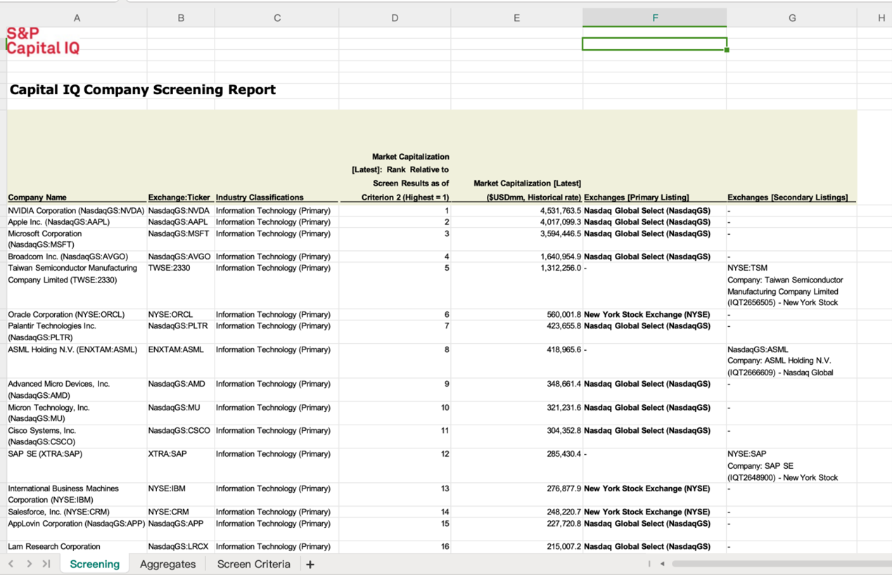
How to define 'TOP 50'? We use the most conspicuous standard: market value. We construct a dictionary through the Screening tool in Capital IQ.
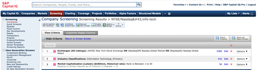
If the stock is listed in not only US market, pay attention that you should only keep its ticker in US. (TSM but not 2330 stands for Taiwan Semiconductor Manufacturing Company, etc.)
Automatical Construction: yfinance
In the latest API update, yfinance may fail to find the "Adj-Close" column due to automatic price adjustment. Therefore, a dynamic detection logic has been added to the code to ensure that the adjusted closing price, which takes into account stock splits and dividends, is obtained.
start_date = "2020-01-01"
end_date = "2025-12-31"
# ban auto_adjust
raw_data = yf.download(tickers, start=start_date, end=end_date, auto_adjust=False, threads=True)
#Prioritize extracting AdjClose (revised price)
available_columns = raw_data.columns.levels[0].tolist()
if 'Adj Close' in available_columns:
    prices = raw_data['Adj Close']
    print("succeed in extracting")
else:
    prices = raw_data['Close']
    print("warning: replacing with 'close'")
#Calculate the daily simple return rate (Returns)
returns = prices.pct_change().dropna(how='all')
prices.to_csv("tech top50 prices.csv")
returns.to_csv("tech top50 returns.csv")
Collecting Social Media Data From Kaggle
After failing to get historical data from Reddit and X (Twitter) directly through APIs, we turn to some existing databases. Here, we found a well established dataset posted on Kaggle.
News&Comments from 2008 to 2024 on Reddit
Part of our code is shown below.
s = df_2020_en["title"].fillna("").astype(str)
# regex for keywords
topic_patterns = {
    k: re.compile(r"\b(?:%s)\b" % "|".join(map(re.escape, v)), flags=re.IGNORECASE)
    for k, v in topic_dict.items()
}
# regex for companies
company_patterns = {
    k: re.compile(r"(?:%s)" % "|".join(map(re.escape, v)), flags=re.IGNORECASE)
    for k, v in company_alias.items()
}
It should be noted that some filtering and merging operations should be added to the code to make the database usable. Here is what we have done.
#Convert the time variables into the same format
df["created_dt"] = pd.to_datetime(df["created"], errors="coerce")
#Filter out titles that contain keywords (i.e. match the regex patterns defined)
topic_hits = pd.DataFrame({k: s.str.contains(pat, na=False) for k, pat in topic_patterns.items()})
company_hits = pd.DataFrame({k: s.str.contains(pat, na=False) for k, pat in company_patterns.items()})
# Need to fit at least one topic pattern or one company pattern
mask_any = topic_hits.any(axis=1) & company_hits.any(axis=1)
df_filtered = df_2020_en.loc[mask_any].copy()
Frequency Count
As we wrote in our first blog, we downloaded the title of related news from Guardian and New York Times. We believe that the message within the news can be well reflected by performing NLP on their titles.
By counting the frequency of specific words written in these titles, we can estimate the media attention on technology companies or news every day. Due to different writing styles of news media, we need to adjust the approach in our code from time to time. Here, we only post an example, so if you are trying to use them in your own project (which is totally welcomed), make sure to its feasibility based on your data sources.
def calculate_daily_frequency(df, column, topic_patterns=topic_patterns, company_patterns=company_patterns, content=0, source=0):
    s = df[column].astype(str)
    # Match topic patterns
    topic_hits = pd.DataFrame({
        k: s.str.contains(pat, na=False)
        for k, pat in topic_patterns.items()
    })
    # Match company patterns
    company_hits = pd.DataFrame({
        k: s.str.contains(pat, na=False)
        for k, pat in company_patterns.items()
    })
    # Match topic pattern and company pattern
    mask_any = topic_hits.any(axis=1) & company_hits.any(axis=1)
    df_filtered = df.loc[mask_any].copy()

    # Calculate total news count per day
    daily_total = (
        df
        .groupby("date")
        .size()
        .rename("total_count")
    )
    # Calculate matched news count per day
    daily_filtered = df_filtered.groupby('date').agg(
        count=(column, 'size'),  # Count news per day
        mean_combined_score=('combined_score', 'mean')
    )
    # Merge results
    daily_counts = (
        daily_total
        .to_frame()
        .join(daily_filtered, how="left")
        .fillna(0)
        .reset_index()
    )
    # Convert types and calculate frequency
    daily_counts["filtered_count"] = daily_counts["count"].astype(int)
    daily_counts["frequency"] = (
        daily_counts["filtered_count"] / daily_counts["total_count"]
    )
    return daily_counts[['date', 'total_count', 'filtered_count', 'frequency', 'mean_combined_score']]
Simple Sentiment Analysis
We combined different kinds of sentiment analysis approaches to better estimate the market sentiment. It includes:
- VADER: Optimized for social media/text with emojis and slang
- TextBlob: Rule-based sentiment analysis with polarity and subjectivity
- Combined Approach: Uses both methods for robust classification
def analyze_sentiment_vader(self, text):
    scores = self.vader_analyzer.polarity_scores(text)
    # Determine sentiment label based on compound score
    compound = scores['compound']
    if compound >= 0.05:
        sentiment_label = 'positive'
    elif compound <= -0.05:
        sentiment_label = 'negative'
    else:
        sentiment_label = 'neutral'
    return {
        'vader_compound': compound,
        'vader_positive': scores['pos'],
        'vader_negative': scores['neg'],
        'vader_neutral': scores['neu'],
        'vader_sentiment': sentiment_label
    }
def analyze_sentiment_textblob(self, text):
    if not text or pd.isna(text):
        return {
            'textblob_polarity': 0,
            'textblob_subjectivity': 0,
            'textblob_sentiment': 'neutral'
        }

    blob = TextBlob(text)

    polarity = blob.sentiment.polarity
    subjectivity = blob.sentiment.subjectivity

    # Determine sentiment label
    if polarity > 0:
        sentiment_label = 'positive'
    elif polarity < 0:
        sentiment_label = 'negative'
    else:
        sentiment_label = 'neutral'

    return {
        'textblob_polarity': polarity,
        'textblob_subjectivity': subjectivity,
        'textblob_sentiment': sentiment_label
    }
Using these approaches, we can simply get a tentative view. We seperated several factors for further analysis:
- Compound Score (-1 to 1): Overall sentiment intensity
- Polarity (-1 to 1): Sentiment direction
- Subjectivity (0 to 1): How opinionated vs factual
- Confidence Score: Agreement between methods
- Categorical Labels: 'positive', 'negative', 'neutral'
TF-IDF Calculation
TF-IDF (Term Frequency-Inverse Document Frequency) is a statistical method used to evaluate the importance of a word in a set of documents. It measures the value of a word in distinguishing documents by multiplying the frequency of the word in a document (TF) with the rarity of the word in the entire corpus (IDF).
We choose this method to better estimate in news, because frequency can only tell part of the story. If a word has a high TF-IDF value, who appears frequently in one article but rarely in other articles, then this word is the "key word" of that particular document. In our project, a higher TF-IDF value indicates that the emotions expressed in this text should be given more weight.
if use_custom_vocab and topic_dict is not None:
     # create a set of keywords
     custom_vocab = set()
     if topic_dict:
         for category, keywords in topic_dict.items():
             for keyword in keywords:
                 # Only keep the keywords that is not long
                 if len(keyword.split()) <= 2:
                     custom_vocab.add(keyword.lower())
     vocabulary = list(custom_vocab)[:max_features]
     print(f"Using custom vocabulary with {len(vocabulary)} terms")
     vectorizer = TfidfVectorizer(
         vocabulary=vocabulary,
         stop_words='english',
         ngram_range=(1, 2),  # allow at most 2-gram
         max_df=0.95,  # ignore the words that appear in 95% of the corpus
         min_df=2,
         norm='l2'
     )
 else:
     # Atomatically extract keywords if no dictionary is provided
     vectorizer = TfidfVectorizer(
         max_features=max_features,
         stop_words='english',
         ngram_range=(1, 2),
         max_df=0.95,
         min_df=2,
         norm='l2'
     )
 # calculate TF-IDF matrix
 tfidf_matrix = vectorizer.fit_transform(corpus)
OLS Regression & Machine Learning
We employed various modeling methods to attempt to link the emotional factors we extracted with the excess returns of technology stocks.
Due to the limited time, we directly downloaded the β value for each stock from Capital IQ, rather than making predictions based on historical data. It might lead to higher estimation error in excess return.
# Prepare dependent and indepedent varaible
X = df[['freq_g_c', 'sent_g_c', 'freq_g_t', 'sent_g_t', 'freq_n_t', 'sent_n_t','freq_r']]
y = df['return']
# Add constant
X = sm.add_constant(X)
# Conduct regression
model = sm.OLS(y, X).fit()
The initial results were not satisfactory. We carefully reviewed the data processing procedure mentioned earlier, corrected some extreme value issues, and attempted to incorporate a time window, which led to more significant regression results. According to our attempts, set the time window to be 4 days after the document is published will obtain a better estimation result.
# Add a time window
result_timewindow = df.copy()
result_timewindow['excess return'] = result_timewindow['excess return'].shift(-4, fill_value=None)
result_timewindow = result_timewindow.dropna()
A series of machine learning models were adopted too, and we try to enhance their performance by adjusting parameters. Here we use Random forest as an example. The R-square result is not as good as OLS.
# Separate features and labels
X = result_timewindow.drop(['date', 'return', 'excess return'], axis=1)  # All TF-IDF features
y = result_timewindow['excess return']
# Split data
X_train, X_test, y_train, y_test = train_test_split(X, y, test_size=0.2, random_state=42)
# Random Forest Regression
rf = RandomForestRegressor(n_estimators=100, random_state=42, n_jobs=-1)
# Simple parameter tuning
param_grid = {
    'max_depth': [5, 10, 20],
    'min_samples_split': [2, 5, 10]
}
grid_search = GridSearchCV(rf, param_grid, cv=3, scoring='r2', n_jobs=-1)
grid_search.fit(X_train, y_train)
# Use best model
best_rf = grid_search.best_estimator_
y_pred_rf = best_rf.predict(X_test)
# Feature importance
feature_importance = pd.DataFrame({
    'feature': X.columns,
    'importance': best_rf.feature_importances_
}).sort_values('importance', ascending=False)
Though our machine learning results are not so ideal, these factor importance may also be enlightening.
Takeaway
After several weeks of trial and adjustment, we initially established a set of Python methods for data acquisition, data cleaning, and extraction of sentiment factors. We then used the extracted factors to attempt to identify their correlations with the stock market. Although our results were not particularly outstanding, we still learned a great many key points:
-
Data means everything. Extracting media data, especially from social media platform could be much more difficult than you imagine. A possible solution is to look for the job done by previous researchers.
-
There is always a way out even in the darkest times. Python is a vast treasure trove. The problem you are currently facing might be troubling someone in another corner of the world. Therefore, make good use of community resources such as GitHub.
-
Sentiment is fleeting. Capturing market sentiment is often very challenging, and investment opportunities derived from historical data analysis may disappear before the code is fully executed.