Introduction
In our second blog post, we dive deeper into our financial sentiment analysis project, building on the foundation laid in our first blog post. During the first part, we applied sentiment analysis to financial news (title) using Large Language Models such as FinBERT, RoBERTa and DeBERTa. After we got the sentiment scores, our group has focused on aggregating sentiment scores by clustering sectors (e.g. technology, finance, energy, etc.) and across the overall market, both in terms of daily frequence. We processed large datasets to create daily sentiment clusters, analyzed sector-specific sentiment trends, and prepared the data for potential time-series analysis to uncover relationships with market movements. This post details our methodology, challenges, and key findings, showcasing how we transformed raw sentiment data into structured, actionable insights.
Data Preprocessing
Our journey began with the raw sentiment data generated from the models (FinBERT, RoBERTa, DeBERTa), where the first two models has "positive score", "neutral score" and "negative score", but the last DeBERTa model only provides "positive" and "negative" scores. Our goal was to aggregate these sentiment scores into meaningful daily clusters, at 1. overall market level and 2. sector level, to enable further time-series analysis. We apply the data preprocessing below:
- Exchange: we select news with all tickers in the following US exchanges: ['NYSE', 'NASDAQ', 'CSE', 'AMEX'] to output US sentiments.
- Time horizon: we filter the data to be after 2017-08-17, because our cryptocurrency data only starts then (from Binance).
- Market value analysis: we filter those tickers with top 80% circulation market value (we want to pay more attention to news from big companies).
Sentiment Clustering Methodology
To aggregate sentiment scores, we developed a custom sentiment_cluster function that addressed two key challenges:
-
Avoiding Double Counting: Some stocks had multiple news articles on the same day, which could skew sentiment scores. We averaged sentiment scores for each stock on a given day to mitigate this.
-
Handling Missing News: For stocks without news on a particular day, we assumed sentiment remained the same as the previous period, using forward-filling to propagate scores.
Here’s a simplified version of our clustering logic:
def sentiment_cluster(df_, stock_counts, analysis_on='finbert', freq='d', impact=3):

    # process column names
    pos_col = analysis_on + '_pos'
    neg_col = analysis_on + '_neg'
    neu_col = analysis_on + '_neu'

    # 1. for the repeated news about the same stock at a certain period, we take the average.
    temp_senti_s = df_.groupby(['ticker', freq_col]).apply(lambda x: x[[pos_col, neg_col, neu_col]].mean(axis=0))

    # 2. stocks have no news remain the same sentiment score as last period.
    temp_senti_freq = temp_senti_s.groupby(level=1).mean()
    temp_count_freq = temp_senti_s.groupby(level=1).apply(lambda x: x.shape[0])
    temp_count_freq.name = 'inner_count'
    temp_merge = pd.concat([stock_counts, temp_count_freq, temp_senti_freq], axis=1).sort_index().ffill()
    cluster_dict = {pos_col: [], neg_col: [], neu_col: []}
    last_senti = {pos_col: temp_merge.head(1)[pos_col].values[0],
                  neg_col: temp_merge.head(1)[neg_col].values[0],
                  neu_col: temp_merge.head(1)[neu_col].values[0]}

    # sentiment daily frequency clustering calculation
    for idx, row in tqdm(temp_merge.iterrows()):
        for s in [pos_col, neg_col, neu_col]:
            temp_put = (row[s] * impact * row['inner_count'] + last_senti[s] * (row['count'] - row['inner_count'])
                           ) / (impact * row['inner_count'] + row['count'] - row['inner_count'])

            cluster_dict[s].append(temp_put)
            last_senti[s] = temp_put
    return pd.DataFrame(data=cluster_dict, index=temp_merge.index)
The impact parameter (set to 3) gave more weight to stocks with news coverage, ensuring that sentiment scores reflected actual news-driven sentiment more heavily than assumed carryover values.
Sector-Specific Clustering
We extended our clustering approach to analyze sentiment by sector using the GICS sector classifications (gsector) in our dataset. For example, "10" represents the "Energy" sector, "40" represents the "Finance" sector, etc. This allowed us to capture sector-specific trends, which are critical for understanding how broader market sentiment might differ across different industries. The sector_cluster function iterated over each sector, applying the same clustering logic:
def sector_cluster(df_, stock_counts_sector):
    sec_dict = {}
    for sector, group in df_.groupby('gsector'):
        cond = stock_counts_sector.index.get_level_values(0) == sector
        tc = stock_counts_sector[cond].reset_index(level=0, drop=True)
        temp_d = sentiment_cluster(group, tc, 'd')
        sec_dict[sector] = temp_d
    return sec_dict
The output was a dictionary of DataFrames, each containing daily sentiment scores for a specific sector. We saved these results as pickled files for future analysis.
Why Sentiment Clustering and Market Proxies?
In our analysis, we aim to transform high-dimensional sentiment scores into a low-dimensional, single value for each day. This transformation is crucial for simplifying the data and making it more interpretable. To achieve this, we aggregate the sentiment scores from individual news articles into a composite score that represents the overall sentiment for each day. This process involves calculating weighted averages of the sentiment scores, taking into account the circulation market value of stocks. By doing so, we ensure that stocks with higher market value have a proportionally greater impact on the overall sentiment score.
Furthermore, we are interested in determining whether our sentiment scores align with the overall market sentiment. To do this, we compare our aggregated sentiment scores with established market sentiment proxies. One such proxy is the "Fear and Greed Index" from CNN, which measures market sentiment based on various factors such as volatility, market momentum, and demand for safe-haven assets. By comparing our sentiment scores with the Fear and Greed Index, we can assess the accuracy and relevance of our sentiment analysis in reflecting broader market trends.
Example output of our clustered sentiment scores
Below is an example of the output of our clustered sentiment scores:
| Index | date | cluster_neg | cluster_pos |
|---|---|---|---|
| 0 | 2017-08-17 | 0.231701 | 0.127091 |
| 1 | 2017-08-18 | 0.199946 | 0.157277 |
| ... | ... | ... | ... |
| 1845 | 2022-09-06 | 0.274161 | 0.186414 |
Comparison between sentiment scores and market proxy
Below is the comparison between our sentiment scores and the market proxy (blue is our sentiment scores, red is the market proxy):
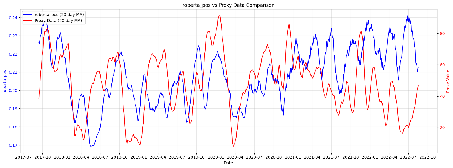
Analysis: The trend observed in our sentiment scores is similar to that of the market proxy. Notably, our sentiment scores tend to lead the market proxy, indicating that our sentiment analysis may provide early signals of market movements.
Developing Sentiment-Driven Trading Strategies
With our aggregated sentiment data in hand, we turned to developing trading strategies to test its predictive power on cryptocurrency markets. We implemented two strategies: sentiment_strategy and moving_average_strategy.
sentiment_strategy: Threshold-Based Trading
The sentiment_strategy function uses sentiment scores as a signal to buy or sell cryptocurrencies. It takes a sentiment factor (e.g., rolling mean of finbert_pos), a cryptocurrency dataset (e.g., BTC, ETH, DOGE, SOL), and buy/sell thresholds (e.g., 0.75). The logic is as follows:
- If the sentiment score falls below a dynamic buy threshold (based on a rolling window), buy (signal=1).
- If the sentiment score exceeds a sell threshold, sell (signal=0).
- Forward-fill positions with a limit to avoid excessive holding periods (
limited_ffill).
We tested this strategy on BTC, DOGE, SOL, and ETH, calculating cumulative returns and visualizing results.
The sentiment_strategy tests whether sentiment extremes (very positive or very negative) can predict short-term price movements in cryptocurrencies. Cryptocurrencies are highly sentiment-driven, making them an ideal testbed for our news-based sentiment signals. By setting dynamic thresholds, we aimed to adapt to changing market conditions and avoid overfitting to static rules.
moving_average_strategy: Trend-Based Trading
The moving_average_strategy applies a classic moving average crossover approach to sentiment scores. It calculates short-term (e.g., 5-day) and long-term (e.g., 20-day) moving averages of the sentiment factor and generates signals:
- Buy (signal=1) when the short-term MA crosses below the long-term MA (indicating a potential reversal).
- Sell (signal=0) when the short-term MA crosses above the long-term MA.
- Compute cumulative returns and plot the results.
We tested this on BTC data, using a factor derived from sector-specific sentiment.
The moving average strategy leverages trends in sentiment rather than absolute levels, aiming to capture momentum shifts. This complements the sentiment_strategy by providing a different perspective on sentiment dynamics. We chose this approach because moving averages are widely used in technical analysis, and applying them to sentiment data allowed us to test whether sentiment trends behave similarly to price trends.
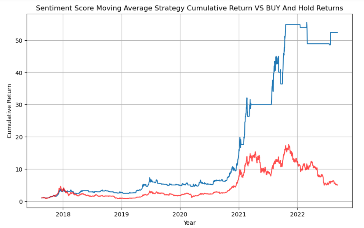
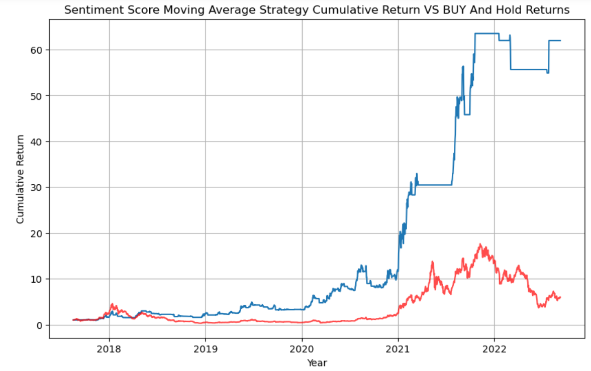
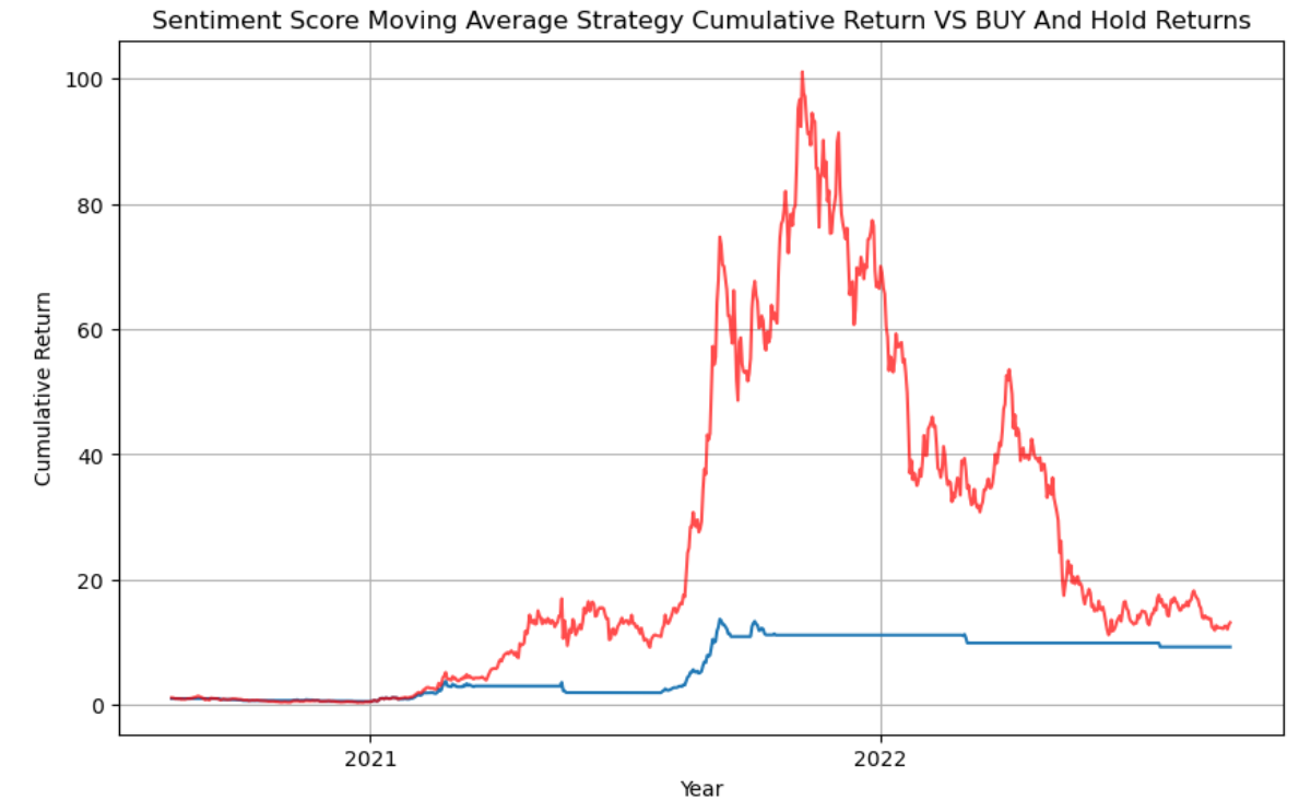
Below are the results of the strategies of Threshold-Based Trading on BTC, ETH, and SOL:
Conclusions
Sentiment Clustering and Market Proxy Integration
- The
finbert_clusterdataset successfully aggregated sentiment scores, reducing noise and providing a stable time series for analysis. - Granger causality tests indicated a statistically significant relationship between
finbert_posand the market proxy at certain lags, suggesting that news sentiment may have predictive power over market sentiment. - Visualizations of
finbert_clusterandsentiment_proxy(20-day rolling means) revealed periods of alignment and divergence, providing qualitative insights into sentiment dynamics.
Trading Strategies
- The
sentiment_strategyproduced varied results across cryptocurrencies. For BTC, cumulative returns showed periods of outperformance, but volatility remained high. Similar patterns emerged for DOGE, SOL, and ETH. - The
moving_average_strategycaptured some sentiment trends but underperformed in highly volatile periods, suggesting that sentiment trends may lag price movements in fast-moving markets like crypto.
Challenges
-
Data Volume and Memory Management: Processing millions of news records (e.g., 13.7 million rows in the FinBERT dataset) required careful memory management. We used
gc.collect()frequently and processed data in chunks where possible. -
Temporal Gaps: Some days had sparse news coverage for certain stocks or sectors, necessitating assumptions about sentiment persistence. While forward-filling helped, it may introduce bias, which we plan to address in future iterations.
-
Model Differences: FinBERT and RoBERTa produced slightly different sentiment distributions, likely due to their training data and tokenization approaches. Reconciling these differences for a unified analysis remains a work in progress.