Thoughts and Processing on Regression Variables (by "Group 9")

By Group "FIN-TANSTIC WIZARDS"

Introduction

In this installment of our GitHub-hosted project, we dive into the preparation of regression variables to analyze the influence of a Social Media Sentiment Divergence Index on Bitcoin’s trading volume and volatility. Having already cleaned the Bitcoin historical data and computed the sentiment divergence index in previous steps, our focus now shifts to defining the variables for regression analysis. This blog explains the process of constructing these variables, the rationale behind our choices, and how we prepared the final dataset for regression. Reflecting on this stage, we realize how much we’ve learned about data manipulation and the importance of thoughtful variable design.

# -*- coding: utf-8 -*-
"""
Spyder Editor

This is a temporary script file.
"""

'''1. Data Cleaning'''
'''pip install pandas numpy openpyxl'''
import pandas as pd
import numpy as np
import openpyxl as opl

Building the Regression Variables

After cleaning the Bitcoin historical data (sourced from Investing.com) and merging it with the sentiment divergence index, we proceeded to create and refine the variables needed for regression. Below is a detailed breakdown of the steps we took. This part of the journey was exciting yet challenging—we initially struggled with understanding how to transform raw financial data into meaningful variables. It took some trial and error to get the formulas right, but we persevered by breaking the problem into smaller steps and consulting documentation.

1. Adding Volatility and Range Metrics

• Daily Returns (Return): We calculated daily returns as a measure of Bitcoin’s price volatility using the formula:
  

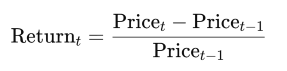
In the code, this was implemented as df['Price'] / df['Price'].shift(-1) - 1, where shift(-1) aligns the previous day’s price. This variable captures the percentage change in price, a standard proxy for volatility in financial studies. We found it tricky at first to align the time series correctly, but adjusting the shift direction solved the issue.

• Price Range (Prange): We introduced Prange to capture intraday volatility, defined as:
  

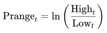
This logarithmic ratio of daily high to low price reflects intraday fluctuations, complementing Return as an alternative volatility measure. The logarithmic transformation was a conceptual leap for us, and we spent time researching why it’s preferred in finance to stabilize variance.

'''1.2 Cleaning Bitcoin Data from Investing.com'''
# Read the CSV file and convert it to a parquet file
csv_file = "Bitcoin historical data.csv"
csv_data = pd.read_csv(csv_file, low_memory=False)  # Prevent warning messages
df = pd.DataFrame(csv_data)
print(df.info())

# Modify data types
df = df.astype(str)

def process_vol(value):
    # Extract numeric value and unit
    num_part = value.replace('B', '').replace('M', '').replace('K', '').replace(',', '')  # Remove B, M, K, or comma
    if num_part == '':
        num_part = pd.NA
        return num_part
    else:
        num = float(num_part)  # Convert to float

    # Adjust value based on unit
    if 'B' in value:
        return num * 1000000000
    elif 'M' in value:
        return num * 1000000
    elif 'K' in value:
        return num * 1000  
    else:
        return num  # Return as is if no unit

for x in ['Price', 'Open', 'High', 'Low', 'Vol.']:
    df[x] = df[x].apply(process_vol)
df[['Date']] = df[['Date']].apply(pd.to_datetime)

# Add variable 'Return', calculated as return_t = (Price_t - Price_t-1) / Price_t-1
df['Return'] = df['Price'] / df['Price'].shift(-1) - 1

# Add variable 'Prange', calculated as prange_t = ln(High_t / Low_t)
df['Prange'] = np.log(df['High'] / df['Low'])

2. Adjusting Trading Volume (aVol)

We created an adjusted volume variable aVol to normalize daily trading volume against its historical average:

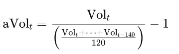
This calculates the current volume relative to a 120-day average (from ( t-140 ) to ( t-21 )), then subtracts 1 to express deviation as a percentage. We chose this approach to account for long-term trends, ensuring the volume reflects relative changes rather than raw magnitudes, which can vary widely over time. The indexing for the 120-day window was a technical hurdle—we had to debug several times to ensure the slice was correctly aligned.

# Add variable 'aVol', calculated as aVol_t = aVol_t / [(aVol_t-21 + ... + aVol_t-140)/120] - 1
df['aVol'] = df['Vol.'] / (df.iloc[df['Vol.'].index[0] + 21 : df['Vol.'].index[0] + 140]['Vol.'].sum() / 120) - 1

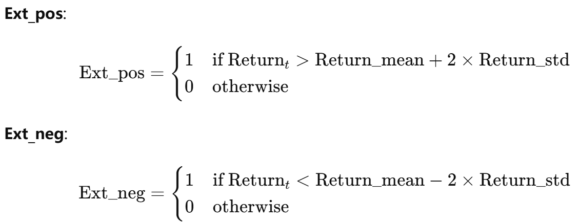
3. Identifying Extreme Returns (Ext_pos and Ext_neg)

To capture extreme market movements, we defined two binary variables: Ext_pos and Ext_neg, indicating days with extremely positive or negative returns:

• Computed the rolling mean (Return_mean) and standard deviation (Return_std) of returns over a 120-day window, shifted with shift(-121).
• Defined:
  This two-standard-deviation threshold identifies outliers often tied to significant market events or sentiment-driven reactions. Implementing the rolling window and applying the conditions was a learning curve—we initially misaligned the shift, but adjusting the -121 offset fixed it.

# Add variables 'Ext_pos' and 'Ext_neg'
# 'Ext_pos' and 'Ext_neg' take the value of 1 for days with extremely positive and negative returns, respectively, and 0 otherwise
df['Return_mean'] = df['Return'].rolling(120).mean().shift(-121)
df['Return_std'] = df['Return'].rolling(120).std().shift(-121)

def Extreme_pos(x):
    if x.Return > x.Return_mean + 2 * x.Return_std:
        return 1
    else:
        return 0

def Extreme_neg(x):
    if x.Return < x.Return_mean - 2 * x.Return_std:
        return 1
    else:
        return 0

df['Ext_pos'] = df[['Return', 'Return_mean', 'Return_std']].apply(Extreme_pos, axis=1)
df['Ext_neg'] = df[['Return', 'Return_mean', 'Return_std']].apply(Extreme_neg, axis=1)

4. Merging with Sentiment Data and User Activity

• Loaded the precomputed sentiment divergence index from daily_sentiment1or-1(2).parquet and saved it as an Excel file (Disagreement.xlsx) for reference. This dataset includes disagt_t, the daily sentiment divergence index.
• Incorporated user activity data from reply_author_count.csv, tracking unique users replying to Bitcoin-related posts. We applied a natural logarithm to the user count (ln_user) to normalize its skewed distribution.
• Merged these datasets with the Bitcoin data using the Date column as the key, using an outer join to retain all data points, then dropped rows with missing values for completeness. Merging datasets was a new challenge—we had to ensure date formats matched, which required some debugging with pd.to_datetime.

'''1.3 Adding Sentiment Divergence Index'''
# Read the Parquet file
df = pd.read_parquet('daily_sentiment1or-1(2).parquet')
print(df.info())
df.to_excel('Disagreement.xlsx')

# Add user count data
csv_file = "reply_author_count.csv"
csv_data = pd.read_csv(csv_file, low_memory=False)  # Prevent warning messages
df_user = pd.DataFrame(csv_data)
print(df_user.info())
df_user[['Reply Author']] = np.log(df_user[['Reply Author']])

# Rename columns: 'Reply Date' to 'Date', 'Reply Author' to 'ln_user'
df1 = df.rename(columns={'Reply Date': 'Date'})
df_user = df_user.rename(columns={'Reply Date': 'Date'})
df_user = df_user.rename(columns={'Reply Author': 'ln_user'})

# Merge Bitcoin data with sentiment divergence data
df_user[['Date']] = df_user[['Date']].apply(pd.to_datetime)
df3 = pd.merge(left=df_by, right=df1, how='outer', on='Date')
df3 = pd.merge(left=df3, right=df_user, how='outer', on='Date')

# Check and remove missing values
print(df3.info())
print(df3.isnull().sum())
df3 = df3.dropna(axis=0, how='any')

# Rename DataFrame and view data summary
df_merge = df3
print(df_merge.info())

5. Finalizing the Regression Dataset

• Dropped unnecessary columns (Price, Open, High, Low, sent_t, Vol., Return_mean, Return_std) that were either intermediate steps or irrelevant to regression. For example, Vol. was replaced by aVol, and raw prices were summarized by Return and Prange.
• Renamed disagt_t to Disagt for clarity and consistency.
• Saved the final dataset—containing Date, Return, Prange, aVol, Ext_pos, Ext_neg, Disagt, and ln_user—as both a Parquet file (Regression variables.parquet) and an Excel file (Regression variables.xlsx) for further analysis. Deciding which columns to drop was a reflective process—we had to weigh their relevance, and we plan to revisit this if the regression reveals unexpected patterns.

'''1.4 Preparing for Regression'''
# Drop variables 'Price', 'Open', 'High', 'Low', 'sent_t', 'Vol.', 'Return_mean', 'Return_std'
df_merge = df_merge.drop(['Price', 'Open', 'High', 'Low', 'sent_t', 'Vol.', 'Return_mean', 'Return_std'], axis=1)

# Rename 'disagt_t' to 'Disagt' and view data summary
df_merge.rename(columns={'disagt_t': 'Disagt'}, inplace=True)
print(df_merge.info())

# Save to current directory
df_merge.to_parquet('Regression variables.parquet')
df_merge.to_excel('Regression variables.xlsx')

Rationale Behind Our Variable Choices

• Multiple Volatility Measures: Using both Return and Prange captures distinct volatility aspects—day-to-day changes versus intraday swings—offering a fuller picture of market dynamics. We chose these after realizing a single measure might miss key patterns.
• Normalized Volume: aVol adjusts for historical trends, isolating relative volume changes potentially driven by sentiment, as raw volumes can reflect market growth over time. This adjustment was a breakthrough after struggling with scale differences.
• Extreme Returns as Indicators: Ext_pos and Ext_neg pinpoint outlier events often linked to sentiment shifts, aiding analysis of whether sentiment divergence amplifies extreme price movements. We found the statistical threshold fascinating and plan to explore alternative thresholds later.
• Log-Transformed User Count: The ln_user transformation addresses skewness in social media activity, ensuring linearity in the regression model. This was a conceptual challenge we overcame by studying data transformation techniques.
• Data Cleaning and Merging: Dropping missing values and irrelevant columns reduces noise and multicollinearity, creating a focused dataset. Reflecting on this, we learned the importance of data quality and intend to refine our cleaning process further.