By Group "Human Superintelligence"
Abstract
This blog focuses on predicting gold prices using Support Vector Machine (SVM) analysis. We first preprocess Reddit comments and other relevant data, conducting sentiment analysis with TextBlob. Then, we build a correlation matrix to explore the relationships between sentiment scores, gold prices, and key market indicators, finding that sentiment scores have limited direct impact on gold prices in the short - term. In the machine learning exploration, we train SVM models with features like sentiment scores, 1 - year interest rates, and VIX. Results show that SVM performs better when combined features are used, with 1 - year interest rates and VIX having a non-linear relationship with gold price returns, while sentiment alone has less predictive power.
1. Data Preprocessing and Sentiment Analysis
Before doing sentiment analysis, we transform raw Reddit comments and replies into structured, analysis-ready data through text cleaning, tokenization, normalization, and feature enrichment (n-grams, NER). Key goals include reducing noise, preserving semantic context, and enhancing machine learning model performance.
def preprocess_text(text):
    """
    Preprocess the text, including word segmentation, removal of stop words, lowercase conversion, Lemmatization, and processing of negative words.
    """
    if not isinstance(text, str):
        return []

    # 1. Tokenization
    tokens = tt.tokenize(text)

    # 2. Stop Word Removal
    filtered_tokens = [word for word in tokens if word.lower() not in stop_words]

    # 3. Lower Case Conversion
    filtered_tokens = [word.lower() for word in filtered_tokens]

    # 4. Lemmatization
    lemmatized_tokens = [wnl.lemmatize(word) for word in filtered_tokens]

    # 5. Handling Negations
    processed_tokens = []
    for i, word in enumerate(lemmatized_tokens):
        if word in negations and i + 1 < len(lemmatized_tokens):
            processed_tokens.append(f"{word}_{lemmatized_tokens[i+1]}")
        else:
            processed_tokens.append(word)

    # 6. Special Words and Named Entity Recognition
    doc = nlp(" ".join(processed_tokens))
    special_tokens = [ent.text.replace(" ", "_") for ent in doc.ents]
    processed_tokens.extend(special_tokens)

    # 7. n-Grams
    bigrams = list(ngrams(processed_tokens, 2))
    trigrams = list(ngrams(processed_tokens, 3))
    processed_tokens.extend([" ".join(bigram) for bigram in bigrams])
    processed_tokens.extend([" ".join(trigram) for trigram in trigrams])

    # 8. Whitespace Elimination
    cleaned_text = ' '.join(processed_tokens).strip()

    return cleaned_text
We selected TextBlob for sentiment analysis after data preprocessing, rather than alternatives like AFINN or VADER, because its polarity scores range continuously from -1 to 1 and exhibit significant variation across different content types. This continuous and nuanced output makes TextBlob better suited for subsequent regression modeling. During sentiment analysis, we identified errors caused by missing values and non-string entries in the dataset. To resolve this, we performed data type validation across all columns, replaced missing values with empty strings, and enforced string formatting for all entries. This preprocessing ensured compatibility with sentiment analysis tools and streamlined the analysis process.
# Check the data type of the column
print(df['Processed Comment'].dtype)
print(df['Processed Reply'].dtype)

# Count the number of non-string values
non_str_maskc = df['Processed Comment'].apply(lambda x: not isinstance(x, str))
print(f"Number of non-string values: {non_str_maskc.sum()}")
non_str_maskr = df['Processed Reply'].apply(lambda x: not isinstance(x, str))
print(f"Number of non-string values: {non_str_maskr.sum()}")

# Fill in null values and convert to string
df['Processed Comment'] = df['Processed Comment'].fillna('').astype(str)
df['Processed Reply'] = df['Processed Reply'].fillna('').astype(str)

df['Comment Sentiment'] = df['Processed Comment'].apply(
    lambda text: TextBlob(text).sentiment.polarity if isinstance(text, str) else 0.0
)
df['Reply Sentiment'] = df['Processed Reply'].apply(
    lambda text: TextBlob(text).sentiment.polarity if isinstance(text, str) else 0.0
)
2. Correlation Matrix Analysis
We first collected and integrated relevant text data and gold price data to build a comprehensive dataset. During data preprocessing, we carefully selected data columns containing sentiment scores, gold prices, and other key indicators that may affect the gold market, and handled missing values rigorously to ensure reliable analysis results. By calculating the correlation matrix, we quantified the linear relationships between these variables, revealing the potential link between sentiment scores and gold prices.
import pandas as pd
import seaborn as sns
import matplotlib.pyplot as plt

# Read the merged data frame
data = pd.read_csv('')

# Select the data columns that need to calculate the correlation.
columns_of_interest = ['Sentiment', 'Open', 'High', 'Low', 'Close', 'Volume', 'Return', 'close_x', 'close_y']
data_subset = data[columns_of_interest]

# Rename columns
data_subset.rename(columns={'close_x': '1-year interest rate', 'close_y': 'vix'}, inplace=True)

# Handle missing values (you can choose to fill them or delete them).
data_subset = data_subset.dropna()

# Calculate the correlation matrix
correlation_matrix = data_subset.corr()
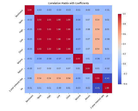
Furthermore, we used visualization techniques to intuitively display these correlations.
# Draw a correlation matrix heatmap
plt.figure(figsize=(10, 8))
sns.heatmap(correlation_matrix, annot=True, fmt='.2f', cmap='coolwarm', square=True, cbar_kws={"shrink": .8})
plt.title('Correlation Matrix with Coefficients')
plt.xticks(rotation=45)
plt.yticks(rotation=45)
plt.tight_layout()
plt.savefig('correlation_matrix_with_coefficients.png')  # Save a correlation matrix heatmap
plt.show()
The following is the visualization result. By analyzing the correlation matrix, we've discovered that the sentiment scores correlate nearly 0 with gold's opening, highest, lowest, and closing prices. This implies limited direct short-term impact of market sentiment on gold prices, or that such impact is overshadowed by stronger market factors. Also, the opening, high, low, and closing prices of gold display a high positive correlation (close to 1), which is expected, as these price indicators represent the same asset's performance at different trading stages, reflecting the gold market's continuity and consistency during transactions. The weak correlation between gold's yield and trading volume suggests that, within our data scope, volume changes don't directly drive significant fluctuations in gold's yield, or their relationship is more complex and influenced by various other factors. Furthermore, the correlation coefficient between the 1-year interest rate and the VIX index is -0.41, indicating a certain negative relationship. This may reflect that during our research period, an increase in interest rates corresponded to a decrease in market volatility expectations and vice versa, a relationship that aligns to some extent with changes in the macroeconomic environment and market risk preferences.
3. Marchine Learning Exploration
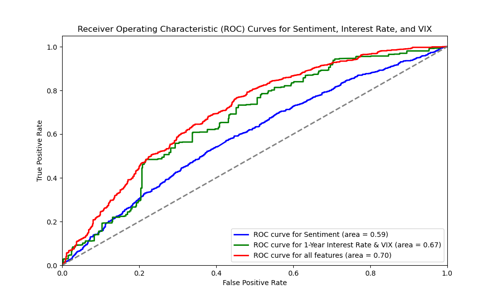
In our exploration of gold price research using machine learning, we delved into Support Vector Machine (SVM) models to uncover potential drivers.We converted gold price returns into binary labels and trained three SVM models based on sentiment scores, 1-year interest rates & VIX, and all features combined. By splitting and standardizing datasets, we ensured scientific training and accurate predictions. The ROC curve served as a crucial tool for evaluating each model's performance in predicting gold price returns, particularly highlighting the role of sentiment factors.
from sklearn.model_selection import train_test_split
from sklearn.svm import SVC
from sklearn.preprocessing import StandardScaler
from sklearn.metrics import roc_curve, auc
import matplotlib.pyplot as plt

# Read the merged dataframe
data = pd.read_csv('')# Convert Return to binary classification labels
y = (data['Return'] > 0).astype(int)

# Feature 1: Only use 'Sentiment'
X_Sentiment = data[['Sentiment']].apply(pd.to_numeric, errors='coerce').dropna()
y_Sentiment = y[X_Sentiment.index]

# Feature 2: 'close_x' and 'close_y'
X_close = data[['close_x', 'close_y']].apply(pd.to_numeric, errors='coerce').dropna()
y_close = y[X_close.index]

# Feature 3: Use all features
X_all = data[['Sentiment', 'close_x', 'close_y']].apply(pd.to_numeric, errors='coerce').dropna()
y_all = y[X_all.index]

# Split the dataset (80% training set, 20% test set) and standardizedef prepare_data(X, y):
    X_train, X_test, y_train, y_test = train_test_split(X, y, test_size=0.2, random_state=5)
    scaler = StandardScaler()
    X_train = scaler.fit_transform(X_train)
    X_test = scaler.transform(X_test)return X_train, X_test, y_train, y_test

# Prepare the data
X_Sentiment_train, X_Sentiment_test, y_Sentiment_train, y_Sentiment_test = prepare_data(X_Sentiment, y_Sentiment)
X_close_train, X_close_test, y_close_train, y_close_test = prepare_data(X_close, y_close)
X_all_train, X_all_test, y_all_train, y_all_test = prepare_data(X_all, y_all)

# Create an SVM model and train it
def train_model(X_train, y_train):
    model = SVC(probability=True)
    model.fit(X_train, y_train)return model

# Train the models
model_Sentiment = train_model(X_Sentiment_train, y_Sentiment_train)
model_close = train_model(X_close_train, y_close_train)
model_all = train_model(X_all_train, y_all_train)

# Make predictions
y_Sentiment_pred_proba = model_Sentiment.predict_proba(X_Sentiment_test)[:, 1]
y_close_pred_proba = model_close.predict_proba(X_close_test)[:, 1]
y_all_pred_proba = model_all.predict_proba(X_all_test)[:, 1]

# Calculate the ROC curve
fpr_Sentiment, tpr_Sentiment, _ = roc_curve(y_Sentiment_test, y_Sentiment_pred_proba)
fpr_close, tpr_close, _ = roc_curve(y_close_test, y_close_pred_proba)
fpr_all, tpr_all, _ = roc_curve(y_all_test, y_all_pred_proba)

roc_auc_Sentiment = auc(fpr_Sentiment, tpr_Sentiment)
roc_auc_close = auc(fpr_close, tpr_close)
roc_auc_all = auc(fpr_all, tpr_all)

# Plot the ROC curve
plt.figure(figsize=(10, 6))
plt.plot(fpr_Sentiment, tpr_Sentiment, color='blue', lw=2, label='ROC curve for Sentiment (area = {:.2f})'.format(roc_auc_Sentiment))
plt.plot(fpr_close, tpr_close, color='green', lw=2, label='ROC curve for 1-Year Interest Rate & VIX (area = {:.2f})'.format(roc_auc_close))
plt.plot(fpr_all, tpr_all, color='red', lw=2, label='ROC curve for all features (area = {:.2f})'.format(roc_auc_all))

plt.plot([0, 1], [0, 1], color='gray', lw=2, linestyle='--')
plt.xlim([0.0, 1.0])
plt.ylim([0.0, 1.05])
plt.xlabel('False Positive Rate')
plt.ylabel('True Positive Rate')
plt.title('Receiver Operating Characteristic (ROC) Curves for Sentiment, Interest Rate, and VIX')
plt.legend(loc='lower right')
plt.savefig('SVM_ROC.png')
plt.show()
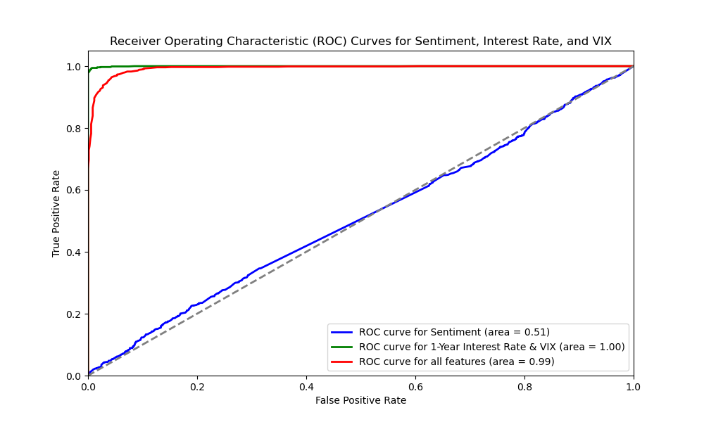
We also experimented with Random Forest models for the same prediction task. Similar to SVM, we built three models using sentiment scores, 1-year interest rates & VIX, and all features. Random Forest excels in handling non-linear relationships and enhances stability through ensemble learning. By training and evaluating these models, we compared their performance and the impact of different features on prediction accuracy.
# Create a Random Forest model and train it
def train_model(X_train, y_train):
    model = RandomForestClassifier(random_state=5)
    model.fit(X_train, y_train)return model

# Train the models
model_Sentiment = train_model(X_Sentiment_train, y_Sentiment_train)
model_close = train_model(X_close_train, y_close_train)
model_all = train_model(X_all_train, y_all_train)
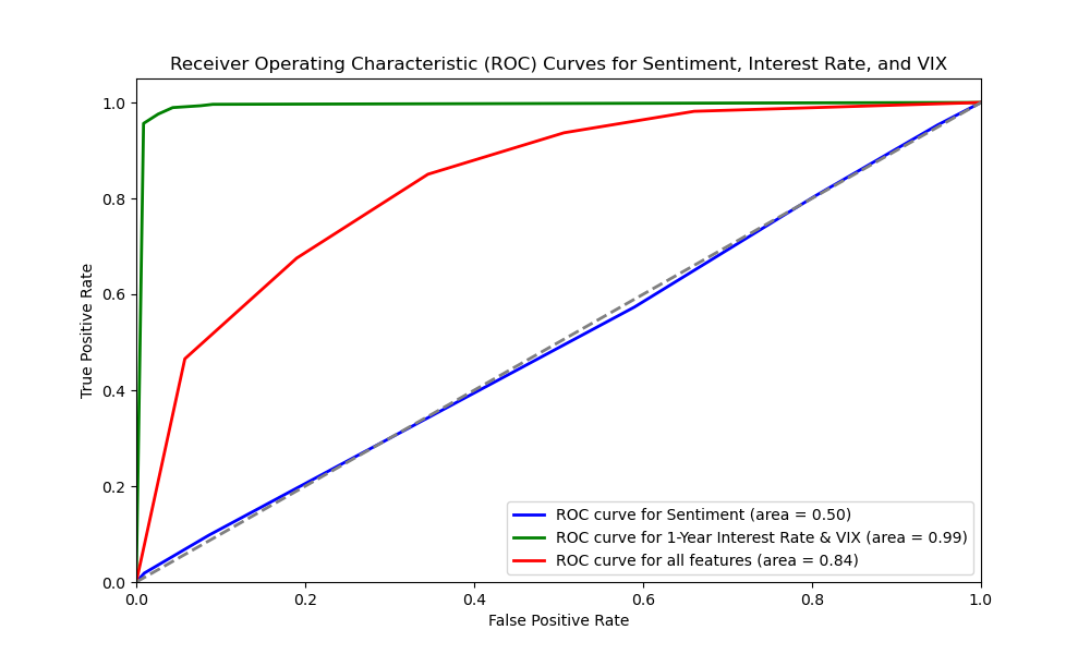
To further explore model applicability, we introduced the K-Nearest Neighbors (KNN) model. This model predicts based on instance similarity, offering simplicity and transparency. We trained three KNN models using the same sets of features and evaluated their performance using ROC curves, adding another dimension to our model comparisons. These diverse machine learning approaches allowed us to comprehensively analyze the complex relationships between gold prices, Reddit sentiment, and other market factors, providing more insightful information for investment decisions and market analysis.
# Create a KNN model and train it
def train_model(X_train, y_train):
    model = KNeighborsClassifier(n_neighbors=5)  # Select an appropriate number of neighbors
    model.fit(X_train, y_train)return model

# Train the models
model_Sentiment = train_model(X_Sentiment_train, y_Sentiment_train)
model_close = train_model(X_close_train, y_close_train)
model_all = train_model(X_all_train, y_all_train)
4. Research Results
In our exploration, we employed various models to predict gold price returns based on sentiment scores, 1-year interest rates & VIX, and all features combined. Our analysis revealed that SVM offered distinct advantages in this context.
The ROC curves showed that SVM had an AUC of 0.59 when using only sentiment scores, indicating limited predictive power from sentiment alone. When using 1-year interest rates & VIX, SVM achieved an impressive AUC of 0.67, demonstrating a non-linear relationship between these market indicators and gold price returns. With all features combined, SVM reached an AUC of 0.70, suggesting that sentiment adds some predictive value but is less influential compared to other factors.
In contrast, Random Forest achieved slightly higher AUC values for sentiment alone (0.51) and 1-year interest rates & VIX (1.00), but slightly lower for all features combined (0.99). This might be due to its sensitivity to noise features in high-dimensional data. KNN showed more balanced performance with AUC values of 0.59, 0.67, and 0.70 respectively, indicating its sensitivity to feature selection and combination.
Considering prediction accuracy and stability, we chose SVM as our primary tool. SVM excels in handling high-dimensional and small-sample data, effectively finding linearly separable hyperplanes even with many features. It also shows robustness to noisy data, making it suitable for volatile financial markets. Through SVM, we gained deeper insights into the complex relationships between gold prices, Reddit sentiment, and other market factors, providing more reliable information for investment decisions and market analysis.