Abstract
This blog employs NLP techniques to empirically examine the impact of sentiment factors derived from corporate earnings call transcripts on stock returns. Following preliminary data collection, we selected transcripts from 10 publicly listed companies spanning four consecutive years as the research sample. Text preprocessing was conducted to eliminate non-standard special symbols, establishing a foundation for subsequent semantic analysis. During the modeling phase, BERT was systematically identified as the core analytical model through comparing against four baseline models. To address overfitting issues between training and validation errors, parameter optimization was implemented, yielding an economically interpretable sentiment score metric.
To evaluate the predictive capacity of sentiment factors in capital markets, we constructed a multivariate regression model incorporating control variables such as firm age, return on equity (ROE), and leverage ratio. Data spanning over 4,000 observations were sourced from Capital IQ and Wind Financial Database for econometric analysis. Empirical results demonstrate a statistically significant positive association (p<0.05) between the extracted sentiment factor and stock returns after rigorous variable controls. This finding provides novel empirical evidence for the textual information pricing theory in behavioral finance, highlighting the materiality of linguistic sentiment signals in financial decision-making.
1. Data Processing
The goal of the data preprocessing work is to merge the three tables downloaded from WRDS through business keys to obtain the standardized data that we will ultimately use for model prediction and subsequent processing.
Firstly, we downloaded the tickers of the constituent stocks of the S&P 500 index from Capital IQ, as well as their company IDs within Capital IQ. Then we filtered out the transcripts IDs corresponding to these stocks.
df_ticker = pd.read_csv('/Users/xingyu/Dropbox/ciq_transcripts/wrds_ticker.csv', sep='\t')

df_stkcd_list = pd.merge(df_stkcd_list, df_ticker, left_on=['Exchange:Ticker', 'Excel Company ID'], right_on=['ticker', 'companyid'], how='left')
df_stkcd_list = df_stkcd_list[['companyname', 'ticker', 'Industry Classifications', 'Excel Company ID', 'startdate', 'enddate']]
df_stkcd_list.rename(columns={'Industry Classifications':'industry', 'Excel Company ID':'companyid'}, inplace=True)

df_stkcd_list = df_stkcd_list[df_stkcd_list['enddate'].isna()]
df_stkcd_list = df_stkcd_list.sort_values(by=['companyname', 'startdate'])
df_stkcd_list = df_stkcd_list.drop_duplicates(subset=['companyname', 'ticker', 'companyid'], keep='first')
Next, we set a series of filters, including stock ticker, transcript type, transcript version, and event date, to filter out the transcript IDs that were precisely suited to our research task.
df_detail = pd.read_csv('/Users/xingyu/Dropbox/ciq_transcripts/wrds_transcript_detail.csv', sep='\t')

companyid_lst = df_stkcd_list['companyid'].tolist()

condition1 = df_detail['companyid'].isin(companyid_lst)
condition2 = df_detail['keydeveventtypename'] == 'Earnings Calls'
condition3 = df_detail['transcriptpresentationtypename'] == 'Final'
condition4 = df_detail['mostimportantdateutc'] >= '2021-01-01'
df_detail = df_detail[condition1 & condition2 & condition3 & condition4]

df_detail = df_detail.sort_values(by=['companyid', 'mostimportantdateutc', 'mostimportanttimeutc', 'transcriptcreationdate_utc', 'transcriptcreationtime_utc'])
df_detail = df_detail.drop_duplicates(subset=['companyid', 'mostimportantdateutc', 'mostimportanttimeutc'], keep='last')
df_detail = df_detail.drop_duplicates(subset=['transcriptid'], keep='last')
Finally, we filtered out the texts corresponding to these transcripts from the ciqtranscriptcomponent table. Due to the length limit of the WRDS database, these texts were segmented at the transcript level. Since many pre-trained models have length input limits, this is also in line with our ultimate goal. In addition, we use a chunk-reading strategy to circumvent the out-of-memory limitation.
file_path = '/Users/xingyu/Dropbox/ciq_transcripts/ciqtranscriptcomponent.csv'

result_df = pd.DataFrame()

transcriptid = df_detail['transcriptid'].tolist()
chunksize = 100000

for chunk in pd.read_csv(file_path, chunksize=chunksize):
    filtered_chunk = chunk[chunk['transcriptid'].isin(transcriptid)]
    result_df = pd.concat([result_df, filtered_chunk], ignore_index=True)

result_df = result_df.sort_values(by=['transcriptid', 'componentorder'])
result_df['transcriptid'] = result_df['transcriptid'].astype(int)

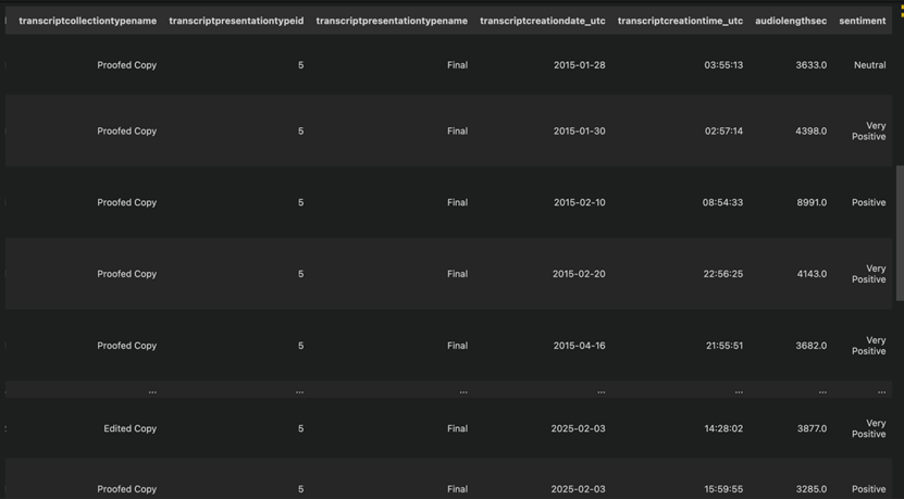
In addition, we also merged the transcripts based on the componentorder key at the transcriptid level to obtain the complete text, and selected one of them to export for cross-checking, which verified that our processing flow was correct and the data quality was high.
merged_df = result_df.groupby('transcriptid').apply(lambda x: '\n'.join(x.sort_values('componentorder')['componenttext'])).reset_index()
merged_df.columns = ['transcriptid', 'componenttext']

text = df.loc[1018, 'componenttext']

with open("/Users/xingyu/Downloads/Apple Inc., Q1 2025 Earnings Call, Jan 30, 2025.txt", "w", encoding="utf-8") as file:
    file.write(text)

2. Model Test
We performed multiple model tests before confirming which model to use for scoring sentiment word classification.
2.1 TabularisAI Machine Model Learning
In one of them, we have loaded TabularisAI multilingual sentiment analysis model by using Hugging Face's Transformers library. The model is based on a Transformer architecture, pre-trained on vast multilingual text corpora (e.g., books, websites, social media). This phase enables it to learn universal language representations, capturing syntactic and semantic patterns across languages. At the same time, we apply a small sample of a separately organized dataset to test it.
2.1.1 Data Preprocessing and Input Handling
We used the code to clean input data by removing rows with missing componenttext. Texts are tokenized using the model's tokenizer, which splits text into subwords, adds padding/truncation to ensure uniform input length (max_length=512), and converts tokens to tensors. This step aligns raw text with the model's expected input format.
# Read the CSV file and make sure the 'componenttext' column is present
df = pd.read_csv(csv_file_path, sep='\t', encoding='utf-8')

# Check if the 'componenttext' column exists
if 'componenttext' not in df.columns:
    raise ValueError("The 'componenttext' column is not found in the CSV file, please check the data format!")

# Load the Transformer Language Model
model_name = "tabularisai/multilingual-sentiment-analysis"
tokenizer = AutoTokenizer.from_pretrained(model_name)
model = AutoModelForSequenceClassification.from_pretrained(model_name)
2.1.2 Inference and Post-processing
The model processes tokenized inputs to generate logits, which are converted into probabilities via softmax. The final sentiment label is assigned by mapping the highest probability class (e.g., index 4 -> "Very Positive") using a predefined sentiment_map.
# Define the sentiment classification function
def predict_sentiment(texts):
    """ Sentiment analysis of texts """
    inputs = tokenizer(texts, return_tensors="pt", truncation=True, padding=True, max_length=512)
    with torch.no_grad():
        outputs = model(**inputs)
    probabilities = torch.nn.functional.softmax(outputs.logits, dim=-1)

    # Setting Emotion Category Mapping
    sentiment_map = {0: "Very Negative", 1: "Negative", 2: "Neutral", 3: "Positive", 4: "Very Positive"}
    return [sentiment_map[p] for p in torch.argmax(probabilities, dim=-1).tolist()]

# Handling of missing values (if there is empty text)
df = df.dropna(subset=['componenttext'])

# Sentiment classification results
df['sentiment'] = predict_sentiment(df['componenttext'].tolist())
df
2.1.3 Results and Limitations
The model provides categorical labels (e.g., "Very Positive", "Positive", "Neutral", etc.), which lack fine-grained sentiment scores that are useful in financial analysis, and thus does not fit our needs. In quantitative finance, analysts often require sentiment scores on a continuous scale (e.g., -1 to +1) instead of broad categories.
2.2 Distilbert-Base-Multilingual-Cased-Sentiments-Model
This model is distilled from the zero-shot classification pipeline on the Multilingual Sentiment dataset.
import pandas as pd
from transformers import pipeline

# Initialize the sentiment analysis pipeline
distilled_student_sentiment_classifier = pipeline(
    model="lxyuan/distilbert-base-multilingual-cased-sentiments-student",
    return_all_scores=True
)

# Get the tokenizer
tokenizer = distilled_student_sentiment_classifier.tokenizer

# Reading the sample(.CSV) file
df = pd.read_csv('temp_data.csv', sep='\t')

# Create new columns to store results
df['positive_score'] = None
df['neutral_score'] = None
df['negative_score'] = None
df['relative_score'] = None

# Define the maximum sequence length
MAX_SEQ_LENGTH = 512

# Perform sentiment analysis on each row of data in the componenttext column in the sample file
for index, row in df.iterrows():
    text = row['componenttext']

    # Tokenization and truncation
    encoded_input = tokenizer.encode_plus(
        text,
        max_length=MAX_SEQ_LENGTH,
        truncation=True,
        return_tensors='pt'
    )

    # Get truncated text from encoded_input
    truncated_text = tokenizer.decode(encoded_input['input_ids'][0], skip_special_tokens=True)

    # Pass truncated text into pipeline for sentiment analysis
    result = distilled_student_sentiment_classifier(truncated_text)

    # Withdrawal Score
    positive_score = result[0][0]['score']
    neutral_score = result[0][1]['score']
    negative_score = result[0][2]['score']
    relative_score = positive_score - negative_score

    # Write to new column
    df.at[index, 'positive_score'] = positive_score
    df.at[index, 'neutral_score'] = neutral_score
    df.at[index, 'negative_score'] = negative_score
    df.at[index, 'relative_score'] = relative_score

# Save the results to a new CSV file
df.to_csv('output.csv', index=False)
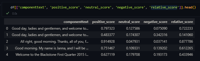
With the model, we can get the probability of Positive, Neutral, and Negative respectively. And by a simple weighting of the three, the relative_score is obtained.
However, the model has a token limit (typically 512 tokens), meaning long earnings call transcripts get truncated, leading to loss of important contextual information. However, Earnings calls often contain detailed discussions, Q&A sessions, and forward-looking statements, which require full context to assess sentiment accurately. This limitation reduces the model's ability to capture sentiment trends across the entire conversation.
3. Model Training
Since the number of output layers of the pre-trained models related to sentiment analysis on Hugging Face is 3, and the open source dataset only has 2 labels, positive and negative, we cannot manually label them due to time and cost constraints. Therefore, we finally chose to fine-tune based on the BERT model.
First, we loaded the data from the dataset and tokenized and preprocessed it to convert it into a format suitable for the torch framework.
from datasets import load_dataset
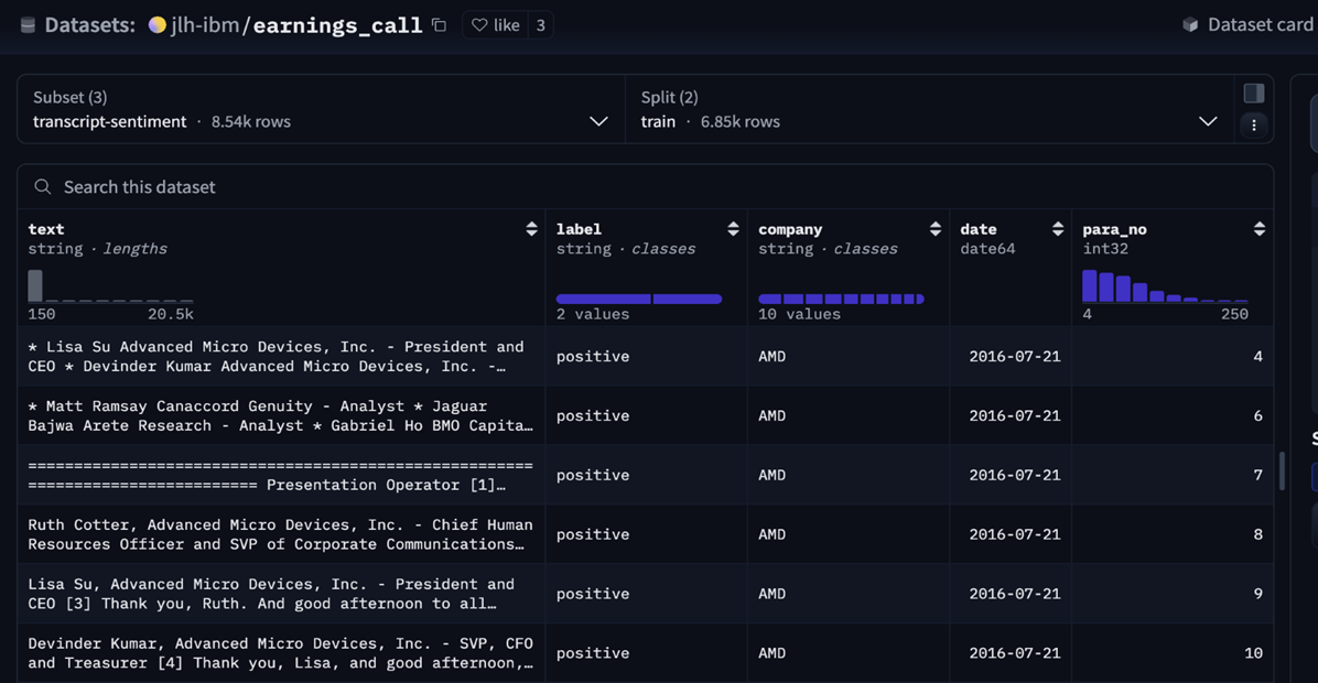
dataset = load_dataset('jlh-ibm/earnings_call', 'transcript-sentiment')
label_map = {'negative': 0, 'positive': 1}
def convert_labels(example):
example['label'] = label_map[example['label']]
return example
dataset['train'] = dataset['train'].map(convert_labels)
dataset['test'] = dataset['test'].map(convert_labels)
def tokenize_function(example):
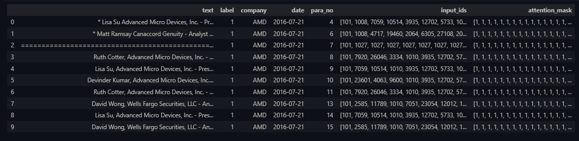
return tokenizer(example['text'], padding='max_length', truncation=True, max_length=256)
tokenized_train_dataset = dataset['train'].map(tokenize_function, batched=True)
tokenized_val_dataset = dataset['test'].map(tokenize_function, batched=True)
tokenized_train_dataset.set_format(type='torch', columns=['input_ids', 'attention_mask', 'label'])
tokenized_val_dataset.set_format(type='torch', columns=['input_ids', 'attention_mask', 'label'])
Next, we fine-tuned Bert on the earnings call dataset and found that around the second epoch, the model started to show a sign of over-fitting. Training loss goes down while validation loss goes up.
from sklearn.metrics import accuracy_score, f1_score
import numpy as np

def compute_metrics(pred):
    labels = pred.label_ids
    preds = np.argmax(pred.predictions, axis=-1)
    acc = accuracy_score(labels, preds)
    f1 = f1_score(labels, preds, average='binary')
    return {'accuracy': acc, 'f1': f1}

bert_model = 'distilbert-base-uncased'
tokenizer = AutoTokenizer.from_pretrained(bert_model)

model = AutoModelForSequenceClassification.from_pretrained('bert-base-uncased', num_labels=2)

training_args = TrainingArguments(
    output_dir='/Users/xingyu/Downloads/temp/results',
    eval_strategy='epoch',
    learning_rate=2e-5,
    per_device_train_batch_size=4,
    per_device_eval_batch_size=4,
    num_train_epochs=4,
    weight_decay=0.01
)

trainer = Trainer(
    model=model,
    args=training_args,
    train_dataset=tokenized_train_dataset,
    eval_dataset=tokenized_val_dataset,
    compute_metrics=compute_metrics
)

trainer.train()
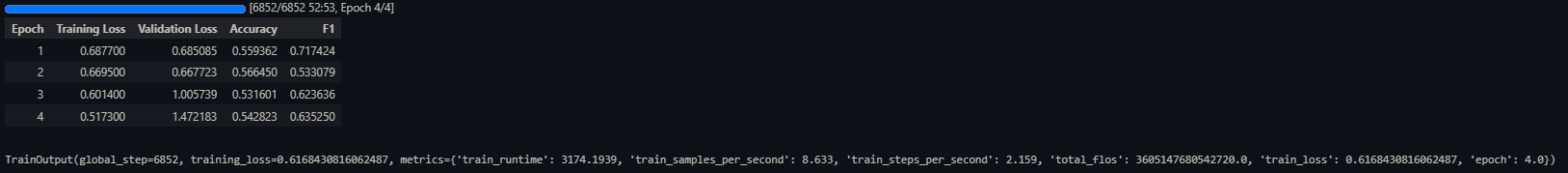
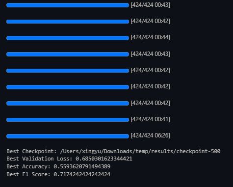
Therefore, we adopted the principle of selecting the model with the smallest validation loss. We evaluated the saved models sequentially using test samples.
best_checkpoint = None
best_accuracy = 0
best_f1 = 0
best_val_loss = float('inf')

checkpoint_dirs = ["/Users/xingyu/Downloads/temp/results/checkpoint-500", "/Users/xingyu/Downloads/temp/results/checkpoint-1000", "/Users/xingyu/Downloads/temp/results/checkpoint-1500", "/Users/xingyu/Downloads/temp/results/checkpoint-2000", "/Users/xingyu/Downloads/temp/results/checkpoint-2500", "/Users/xingyu/Downloads/temp/results/checkpoint-3000", "/Users/xingyu/Downloads/temp/results/checkpoint-3500", "/Users/xingyu/Downloads/temp/results/checkpoint-4000", "/Users/xingyu/Downloads/temp/results/checkpoint-4500"]

for checkpoint_dir in checkpoint_dirs:

    model = AutoModelForSequenceClassification.from_pretrained(checkpoint_dir)

    trainer = Trainer(
        model=model,
        args=training_args,
        eval_dataset=tokenized_val_dataset,
        compute_metrics=compute_metrics
    )

    eval_results = trainer.evaluate()

    if eval_results['eval_loss'] < best_val_loss:
        best_val_loss = eval_results['eval_loss']
        best_checkpoint = checkpoint_dir
        best_accuracy = eval_results['eval_accuracy']
        best_f1 = eval_results['eval_f1']

print(f"Best Checkpoint: {best_checkpoint}")
print(f"Best Validation Loss: {best_val_loss}")
print(f"Best Accuracy: {best_accuracy}")
print(f"Best F1 Score: {best_f1}")
And we selected the optimal one for the prediction of S&P 500 index component stocks from 2021 to 2024 based on WRDS high quality text.
model = AutoModelForSequenceClassification.from_pretrained("/Users/xingyu/Downloads/temp/results/checkpoint-500")

trainer = Trainer(
    model=model,
    args=training_args,
    eval_dataset=tokenized_val_dataset
)

predictions = trainer.predict(tokenized_predict_dataset)
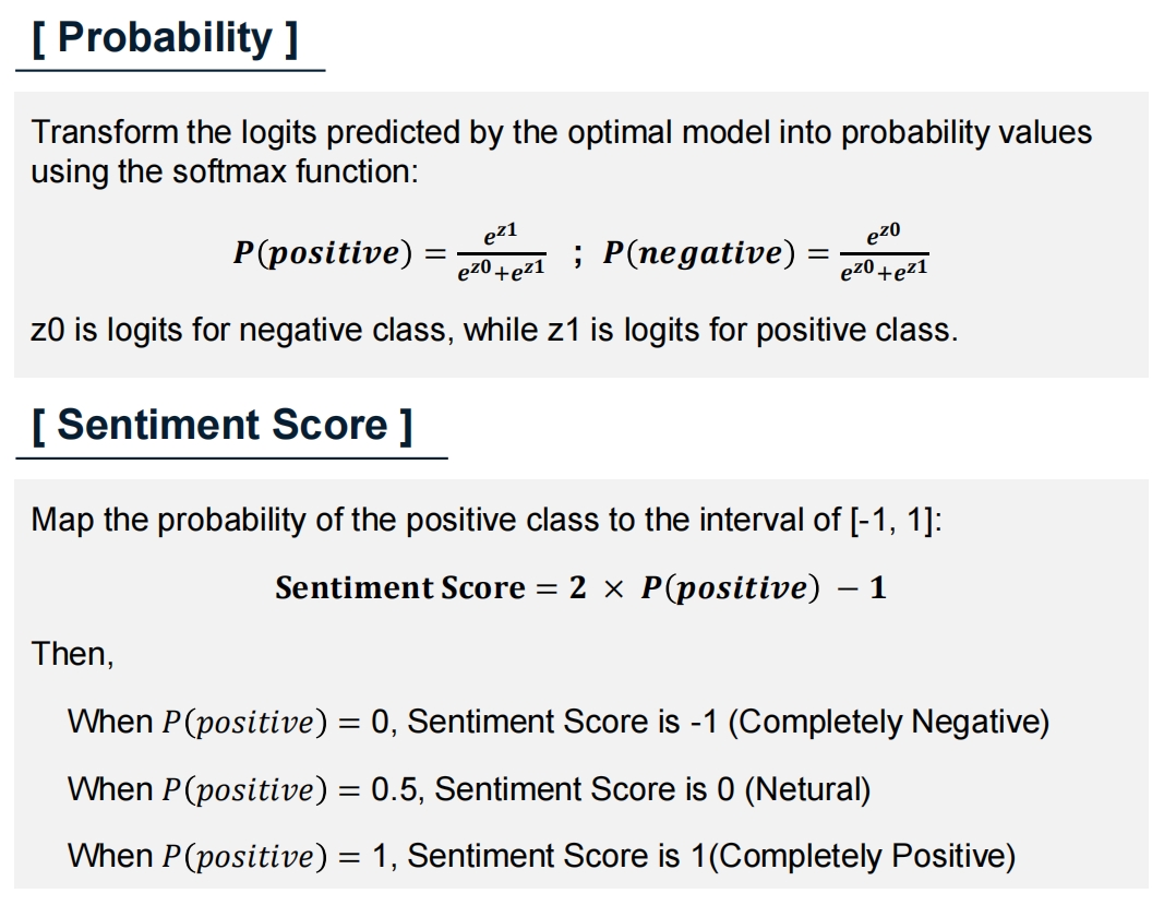
Once we had our predictions, we used the softmax function to turn the raw logits into probabilities. Then, we mapped the probability of the positive class to a range between minus one and one, which gave us a sentiment score for each sentence. Finally, these scores were equally weighted and summed at the transcript level to derive the overall sentiment score.
4. Regression
4.1 Sample Selection and Data Processing
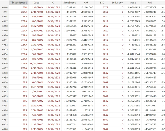
We selected S&P 500 constituent stocks as our sample, taking excess returns of the S&P 500 as the dependent variable. The sentiment factor constructed from earnings call transcripts serves as the independent variable. We also included company age, ROE, leverage ratio, asset turnover, institutional ownership, employee size, and revenue growth rate as control variables. The analysis spans the period from 2021 to 2023. Company age and revenue growth rate data are sourced from Wind, while all other data are obtained from Compustat and Capital IQ within the CRSP database. After removing all missing values, a total of 4,970 observations were obtained.
4.2 Variable Processing
4.2.1 Dependent Variable (CAR) Processing
We computed the cumulative abnormal returns (CAR) for three days before and after the earnings call to assess the short-term effect of sentiment expressed during earnings calls on stock returns.
import pandas as pd
def process_earnings_calls(earnings_file, returns_file, output_file):
    earnings_df = pd.read_csv(earnings_file)
    returns_df = pd.read_excel(returns_file)

    # Ensure that dates are formatted correctly
    earnings_df["mostimportantdateutc"] = pd.to_datetime(earnings_df["mostimportantdateutc"], format="%Y/%m/%d")
    returns_df["Date"] = pd.to_datetime(returns_df["Date"], format="%Y/%m/%d")

    # Grouping data by company code
    returns_df = returns_df.sort_values(by=["Ticker Symbol", "Date"]).reset_index(drop=True)
    grouped_returns = returns_df.groupby("Ticker Symbol")

    # Results
    results = []
    for _, row in earnings_df.iterrows():
        ticker = row["ticker"]
        event_date = row["mostimportantdateutc"]
        if ticker not in grouped_returns.groups:
            continue  # If the company is not in the daily excess returns, skip it.

        # Access to the company's data
        company_data = grouped_returns.get_group(ticker).reset_index(drop=True)
        dates = company_data["Date"]

        # Find the closest trading day index
        idx = dates.searchsorted(event_date)
        if idx == len(dates) or dates.iloc[idx] != event_date:
            idx -= 1  # If event_date is not a trading day, take the index before the most recent trading day.

        # Make sure the index is valid
        if idx < 0:
            continue  # If the index is not legal, skip

        # Calculate the sum of the excess returns of the first 3 days + the current day + the next 3 days
        start_idx = max(0, idx - 3)
        end_idx = min(len(dates) - 1, idx + 3)
        excess_return_sum = company_data.loc[start_idx:end_idx, "daily excess return"].sum()

        # Record results
        results.append([ticker, event_date.strftime("%Y/%m/%d"), excess_return_sum])

    # Save results
    result_df = pd.DataFrame(results, columns=["ticker", "mostimportantdateutc", "7_day_excess_return_sum"])
    result_df.to_csv(output_file, index=False)
    print(f" The results have been saved to {output_file}")

# Call function
process_earnings_calls("earnings_calls_date.csv", "daily excess returns.xlsx", "processed_results.csv")
4.2.2 Independent Variable (Sent) Processing
Since our constructed sentiment factors are predominantly positive, we standardized sentiment scores at the company level to measure the relative changes in sentiment during earnings calls and their impact on stock prices.
# Sentiment standardization by company
df['Sentiment_Z2'] = df.groupby('TickerSymbol')['Sentiment'].transform(lambda x: (x - x.mean()) / x.std())
4.3 Empirical Analysis
In this part, We did some necessary analyses prior to the regression, including correlation test and multicollinearity analysis. And the results of baseline regression illustrate a significantly positive relationship between stock excess returns and earnings call sentiment.
4.3.1 Correlation Test
# Correlation test
corr_matrix = df[['CAR', 'Sentiment_Z2', 'age1', 'ROE', 'SalesGrowthRate',
                  'employernumber', 'TotalInstOwnershipPercento', 'AssetTurnover', 'Q']].corr()
print("\nCorrelation:")
print(corr_matrix)
4.3.2 Multicollinearity Analysis
# Test for multicollinearity (VIF)
def calculate_vif(data):
    vif_data = pd.DataFrame()
    vif_data["Variable"] = data.columns
    vif_data["VIF"] = [variance_inflation_factor(data.values, i) for i in range(data.shape[1])]
    return vif_data

# Extraction of independent variables
X = df[['Sentiment_Z2', 'age1', 'ROE', 'SalesGrowthRate', 'employernumber',
        'TotalInstOwnershipPercento', 'AssetTurnover', 'Q']]
X = sm.add_constant(X)

# Calculate VIF
vif_results = calculate_vif(X)
print("\nMulticollinearity()VIF):")
print(vif_results)
4.3.3 Baseline Regression
# Regression 1: Simple regression
model1 = ols('CAR ~ Sentiment_Z2', data=df).fit()
print("\nRegression1:")
print(model1.summary())

# Regression 2: Fixed effects regression (absorption of SIC and C)
df['C'] = pd.to_datetime(df['C'])
df = df.set_index(['SIC', 'C'])  # Setting the panel data index
model2 = PanelOLS.from_formula('CAR ~ Sentiment_Z2 + EntityEffects + TimeEffects', data=df)
results2 = model2.fit(cov_type='clustered', cluster_entity=True)
print("\nRegression2:")
print(results2.summary)

# Regression 3: Multiple regression
model3 = ols('CAR ~ Sentiment_Z2 + age1 + ROE + SalesGrowthRate + employernumber + TotalInstOwnershipPercento + AssetTurnover + Q', data=df).fit()
print("\nRegression3:")
print(model3.summary())

# Regression 4: Fixed-effects multiple regression (absorbing SIC and C)
model4 = PanelOLS.from_formula('CAR ~ Sentiment_Z2 + age1 + ROE + SalesGrowthRate + employernumber + TotalInstOwnershipPercento + AssetTurnover + Q + EntityEffects + TimeEffects', data=df)
results4 = model4.fit(cov_type='clustered', cluster_entity=True)
print("\nRegression4:")
print(results4.summary)
4.3.4 Extensive Analysis
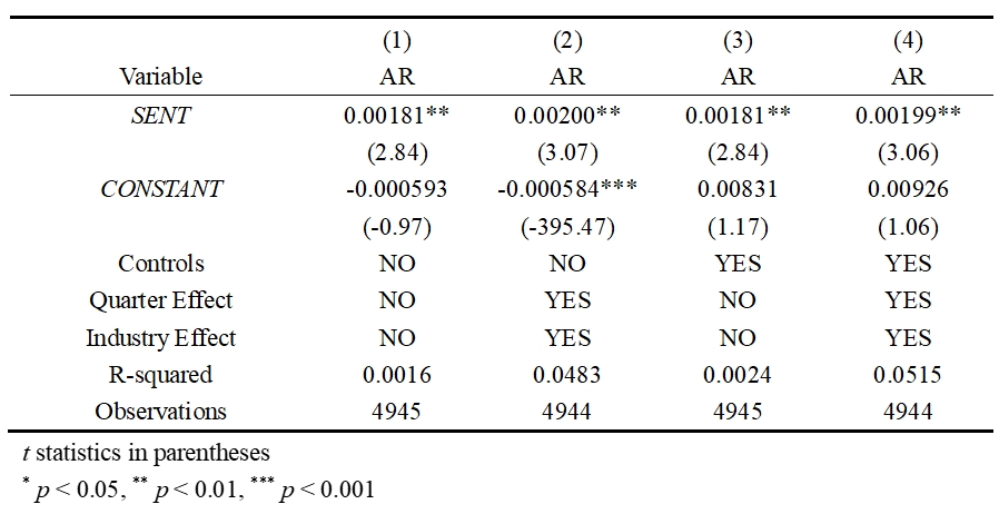
During the final class presentation, Professor Buehlmaier suggested performing a robustness check by using the abnormal returns on the day of the earnings call as the dependent variable. We incorporated this suggestion and conducted the analysis accordingly.
# Regression analysis - Robustness Test with abnormal daily excess returns
# Regression 5: Simple regression
model5 = ols('AR ~ Sentiment_Z2', data=df).fit()
print("\nRegression5:")
print(model5.summary())

# Regression 6: Fixed effects regression (absorption of SIC and C)
df['C'] = pd.to_datetime(df['C'])
df = df.set_index(['SIC', 'C'])  # Setting the panel data index
model6 = PanelOLS.from_formula('AR ~ Sentiment_Z2 + EntityEffects + TimeEffects', data=df)
results6 = model6.fit(cov_type='clustered', cluster_entity=True)
print("\nRegression6:")
print(results6.summary)

# Regression 7: Multiple regression
model7 = ols('AR ~ Sentiment_Z2 + age1 + ROE + SalesGrowthRate + employernumber + TotalInstOwnershipPercento + AssetTurnover + Q', data=df).fit()
print("\nRegression7:")
print(model7.summary())

# Regression 8: Fixed-effects multiple regression (absorbing SIC and C)
model8 = PanelOLS.from_formula('AR ~ Sentiment_Z2 + age1 + ROE + SalesGrowthRate + employernumber + TotalInstOwnershipPercento + AssetTurnover + Q + EntityEffects + TimeEffects', data=df)
results8 = model8.fit(cov_type='clustered', cluster_entity=True)
print("\nRegression8:")
print(results8.summary)
The extensive analysis results remain significant, providing further support for our initial hypothesis.
4.4 Why Python and Stata Regression Results May Differ
We have found some differences in the regression results output with Stata and Python for the same dataset. Therefore, consider the following possible reasons:
-
Data Handling Differences
- Missing Values: Stata automatically excludes missing values in regression, while Python requires explicit handling (e.g., dropna()).
- Data Types: Stata may automatically recognize categorical variables, whereas Python requires explicit conversion (e.g., astype('category')).
- Standardization: Differences in standardization formulas (e.g., sample standard deviation in Stata vs. population standard deviation in Python).
-
Algorithmic Differences
- Optimization Methods: Stata and Python may use different optimization algorithms or convergence criteria for estimating regression models.
- Numerical Precision: Differences in numerical precision or rounding errors can lead to small discrepancies in results.
-
Statistical analysis Differences
- Stata professional statistical accuracy: built-in extremely rich and mature statistical analysis program package, in economics, sociology and other fields use Stata.
- Python statistical expertise is slightly weaker: the statistical module output is not as fine as Stata, and traditional statistical analysis is less convenient, but more versatile when dealing with large amounts of data, cross-domain projects, and customized algorithms.