By Group "Fintext"
Understanding the relationship between textual signals in corporate disclosures and market behavior represents a critical area of financial NLP research. This study proposes a systematic methodology to extract and quantify sentiment signals from 10-K filings using FinBERT, evaluating their potential associations with long-term equity performance through multi-year buy-and-hold return analysis. Our framework combines advanced NLP techniques with financial econometrics to investigate whether document-level sentiment patterns in mandatory disclosures exhibit measurable correlations with subsequent stock returns. This exploratory approach contributes to financial informatics literature by demonstrating a replicable pipeline for analyzing corporate communication effects while providing practical insights into text-based market signal extraction.
Part 4: Sentiment Analysis with FinBERT
In this step, we will analyze the sentiment of the extracted text from the 10-K reports using the FinBERT model, specifically designed for financial data. This process involves several key tasks, from loading the text files to processing the sentiment scores and saving the results in a structured format.
Loading and Processing the Repodrts
We begin by loading the necessary libraries and the FinBERT model. The model will enable us to classify the sentiment of the text into positive, negative, and neutral categories.
import os
import glob
import pandas as pd
from transformers import AutoTokenizer, AutoModelForSequenceClassification
import torch

# Load FinBERT
tokenizer = AutoTokenizer.from_pretrained("yiyanghkust/finbert-tone")
model = AutoModelForSequenceClassification.from_pretrained("yiyanghkust/finbert-tone")
Reading and Splitting Text
Next, we define functions to read the text files and split the text into manageable chunks. This is essential because FinBERT has a maximum input size, and we want to ensure that we do not exceed this limit.
def load_text(file_path):
    with open(file_path, "r", encoding="utf-8") as f:
        return f.read()

def split_text(text, chunk_size=300):
    words = text.split()
    return [" ".join(words[i:i+chunk_size]) for i in range(0, len(words), chunk_size)]
Sentiment Analysis
Sentiment Analysis
The core of our analysis lies in the analyze_sentiment function. For each chunk of text, we use FinBERT to predict the sentiment scores, which are then aggregated to compute the total positive, negative, and neutral scores.
def analyze_sentiment(text_chunks):
    total_positive, total_negative, total_neutral = 0, 0, 0

    for chunk in text_chunks:
        inputs = tokenizer(chunk, return_tensors="pt", truncation=True, max_length=512)
        outputs = model(**inputs)
        scores = torch.nn.functional.softmax(outputs.logits, dim=-1)  # Softmax to get probabilities

        total_negative += scores[0][0].item()
        total_neutral += scores[0][1].item()
        total_positive += scores[0][2].item()

    return total_positive, total_negative, total_neutral
Conclusion
This step successfully leverages the FinBERT model to analyze the sentiment of 10-K reports, providing valuable insights into the overall sentiment conveyed in corporate communications. By extracting sentiment scores and ratios, we set the stage for further analysis, allowing us to track sentiment trends over time and correlate them with financial performance.
Part 5: Comparing Sentiment Scores Over the Years
In this section, we will evaluate the relationship between sentiment changes and stock performance by defining a function to calculate buy-and-hold returns and then validating our findings through analysis.
Defining the Buy-and-Hold Return Function
First, we define a function to calculate the buy-and-hold return for a given stock over a specified holding period. This function ensures that the start and end dates are valid trading days.
def calculate_returns(df, stock_ticker, start_date='2019-01-01', hold_period_days=2192):
    start_date = pd.to_datetime(start_date)
    end_date = start_date + pd.Timedelta(days=hold_period_days)

    # Ensure the DataFrame index is a DatetimeIndex
    if not isinstance(df.index, pd.DatetimeIndex):
        df.index = pd.to_datetime(df.index)

    # Adjust start_date to the next available trading day if necessary
    if start_date not in df.index:
        while start_date not in df.index:
            start_date += pd.Timedelta(days=1)

    # Adjust end_date to the next available trading day if necessary
    if end_date not in df.index:
        while end_date not in df.index:
            end_date += pd.Timedelta(days=1)

    # Get the prices for the adjusted dates
    start_price = df.loc[start_date, stock_ticker]
    end_price = df.loc[end_date, stock_ticker]

    # Calculate buy-and-hold return
    buy_hold_return = ((end_price / start_price) - 1)

    return buy_hold_return.round(4)  # Round to 4 decimal places
Defining the Buy-and-Hold Return Function
Next, we will validate our findings by grouping companies based on their positive_ratio_diff for each year. We will separate them into high-change and low-change groups, then calculate the average buy-and-hold return for each group to see if there is a correlation between sentiment changes and stock performance.
returns = []
for year, group in senti.groupby('year'):
    group = group.sort_values(by='positive_ratio_diff', ascending=False)

    # Separate into high-change and low-change groups
    mid_index = len(group) // 2
    high_group = group.iloc[:mid_index]
    low_group = group.iloc[mid_index:]

    # Calculate average return for high-change group
    high_returns = []
    for index, row in high_group.iterrows():
        return_value = calculate_returns(close_dfs[row['stock']], row['stock'], start_date=row['date'], hold_period_days=6)
        high_returns.append(return_value)

    # Calculate average return for low-change group
    low_returns = []
    for index, row in low_group.iterrows():
        return_value = calculate_returns(close_dfs[row['stock']], row['stock'], start_date=row['date'], hold_period_days=6)
        low_returns.append(return_value)

    # Record the results
    returns.append({
        'year': year,
        'high_avg_return': np.mean(high_returns),
        'low_avg_return': np.mean(low_returns)
    })

# Convert results to DataFrame for analysis
returns_df = pd.DataFrame(returns)
print(returns_df)
Conclusion
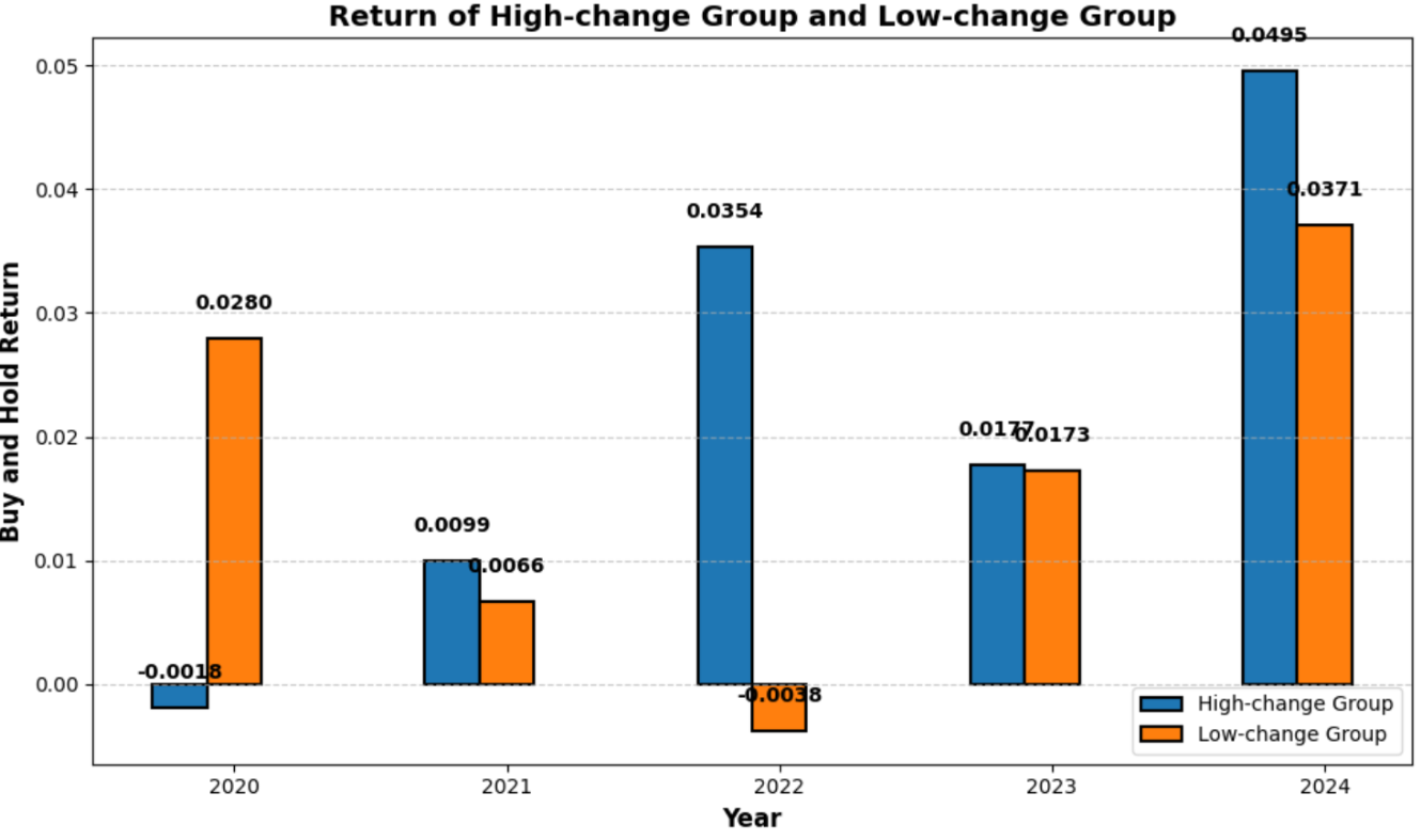
Through these analyses, we can observe whether sentiment changes, particularly in the positive ratios, correlate with stock performance across different companies and years. The figure below demonstrates the average weekly buy-and-hold return of high-change group and low-change group after the release of the 10-k report. In 4 out of 5 years, the group with more positive sentiment changes has a higher return, which supports our hypothesis that the stock price is likely to increase after the company issues a more positive 10-k report than the report issued last year.
This method provides valuable insights for investors looking to make informed decisions based on market sentiment trends. By understanding the relationship between sentiment and stock returns, investors can better strategize their investments.
Part 6: Future Improvement
Finally, we will discuss potential improvements for achieving better results in sentiment analysis. After presenting our data analysis in class, we received valuable feedback from our professor that can enhance the accuracy. Here are a few key points for future improvements:
-
Model Fine-Tuning: Leveraging the outputs from the FinBERT model to fine-tune it with our specific dataset of 10-K reports can significantly enhance its accuracy. This approach allows the model to better understand the nuances of financial language and improve sentiment predictions tailored to our context.
-
Expanding the Dataset: Incorporating a larger and more diverse dataset for training, including additional financial documents and relevant news articles, can improve the model's robustness. A richer dataset will help the model generalize better and capture various sentiment expressions in financial contexts.
-
Integration with Other Data Sources: Combining sentiment scores with other financial metrics—such as stock price movements, trading volumes, and market trends—can provide a more comprehensive analysis. This integration will enable us to better understand the relationship between sentiment and market behavior, offering deeper insights for investors and stakeholders.