Introduction
In our first blog, we detailed the processes of data collection, preprocessing, and the generation of word clouds to present our progressive results. We obtained the federal funds rate data from the Federal Reserve Bank of St. Louis website and sourced text data from FOMC statements, minutes, SEP reports, and public speeches by officials via the official website of the Federal Reserve. Our preprocessing steps included tokenization, conversion to lowercase, removal of punctuation and stop words, as well as stemming and lemmatization. Following these steps, we established two SQLite databases for further analysis.
Over time, we have employed machine learning to train a model to predict the target federal funds rate using FOMC texts. This blog will focus on the two frameworks we used to train the model and the validation of their accuracy.
Framework 1: FinBERT + LSTM Neural Network
Sentiment Analysis: FinBERT
After reviewing relevant literature, we decided to utilize the FinBERT model for sentiment analysis. FinBERT is a BERT model specifically optimized for financial domain texts, offering high accuracy and practicality.
To start, we defined a class named FinBertSentimentAnalyzer. The code we use is as follows:
class FinBertSentimentAnalyzer:
    def __init__(self):
        self.tokenizer = AutoTokenizer.from_pretrained("ProsusAI/finbert")
        self.model = AutoModelForSequenceClassification.from_pretrained("ProsusAI/finbert")
        self.device = 0 if torch.cuda.is_available() else -1
        self.classifier = pipeline(
            "text-classification",
            model=self.model,
            tokenizer=self.tokenizer,
            device=self.device
        )
        self.max_seq_length = 512
Viewing that FinBERT has an inherent constraint of limiting input text length to 512 tokens due to its BERT architecture, we designed a chunk_text function to handle longer texts. The code we use is as follows:
def _chunk_text(self, text):
    """"split long text into segments suitable for model processing"""
    words = text.split()
    chunks = []
    current_chunk = []

    # intelligent chunking based on words and punctuation
    for word in words:
        if len(' '.join(current_chunk + [word])) < self.max_seq_length:
            current_chunk.append(word)
        else:
            chunks.append(' '.join(current_chunk))
            current_chunk = [word]
    if current_chunk:
        chunks.append(' '.join(current_chunk))
    return chunks
Most importantly, we wrote code to perform sentiment analysis on the input text and return a composite score. First, we split the input text into multiple chunks that were suitable for processing by the model. If no chunks were generated, we returned 0.0, indicating a neutral sentiment. Next, we iterated through each chunk and used a pre-trained sentiment analysis classifier to analyze it. The analysis results included a sentiment label and its corresponding score. Based on the sentiment label, we converted the score into numerical values: positive sentiment scores were positive, negative sentiment scores were negative, and neutral sentiment scores were 0. If we encountered an error while processing a chunk, we logged the error and set the score to 0. Finally, we calculated the weighted average of all the scores and returned the overall sentiment score. If there were no scores, we returned 0.0. The code we use is as follows:
def analyze_sentiment(self, text):
    """Perform sentiment analysis and return a composite score."""
    chunks = self._chunk_text(text)
    if not chunks:
        return 0.0  # Return neutral for empty text

    scores = []
    for chunk in chunks:
        try:
            result = self.classifier(chunk)[0]
            # Convert labels to numerical values: positive=1, negative=-1, neutral=0
            if result['label'] == 'positive':
                scores.append(result['score'])
            elif result['label'] == 'negative':
                scores.append(-result['score'])
            else:
                scores.append(0)
        except Exception as e:
            print(f"Error processing chunk: {str(e)}")
            scores.append(0)

    # Calculate the final score as a weighted average
    return sum(scores) / len(scores) if scores else 0.0
To our surprise, when we applied the model to our processed data in the first blog, the results were predominantly neutral, with most values clustering around zero. After conducting further research, we discovered that FinBERT has its own tokenization process, and using unprocessed text yielded more varied results. Consequently, we refined our data preprocessing approach by only removing special characters and redundant spaces, while also addressing common formatting issues. When we applied the model to the newly processed data, the scores varied more widely and appeared more normal.
Model: LSTM Neural Network
Data Preparation
Above all, we needed to perform additional data processing to obtain a one-to-one feature matrix and target variable.
To clarify, we selected the Upper Limit of the Target Fed Funds Rate every seven weeks as our target variable, since the Target Fed Funds Rate was typically published every seven weeks, and we used the Sentiment Analysis Scores from FinBERT to create the feature matrix.
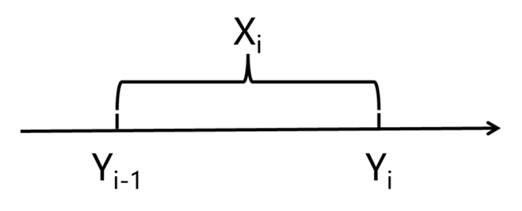
For the feature matrix, we aligned the sentiment scores with the corresponding Fed Funds Rate dates, as shown in the following picture. In this representation, X denotes a list of sentiment scores, while Y represents the Fed Funds Rate.
After the above alignment, the result is shown in the following picture.
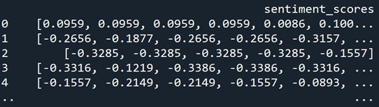
Next, we padded the shorter lists in the DataFrame with zeros to match the maximum length. Then, we converted these padded lists into a numpy array for model input. Since zeros indicated neutrality, we believed this approach was acceptable. Finally, we obtained the feature matrix. The code we use is as follows:
# Convert the sentiment_scores column to a numerical matrix
max_length = X['sentiment_scores'].apply(len).max() # Find the length of the longest list
X = np.array(X['sentiment_scores'].apply(lambda x: x + [0] * (max_length - len(x))).tolist())  # Pad with 0s
For the target variable, we classified Fed Funds Rate changes into three categories: Increase, Decrease, or No Change. The code we use is as follows:
y = pd.Series(selected_rates)
y_diff = y.diff().dropna()  # Difference and remove the first NaN value
y_labels = np.sign(y_diff)  # 1: positive, -1: negative, 0: zero
# Convert classification labels to one-hot encoding
y_labels = to_categorical(y_labels + 1, num_classes=3)  # Map -1, 0, 1 to 0, 1, 2
Model Architecture
Our model was based on an LSTM neural network. We chose LSTM because our data exhibited temporal dependencies, and LSTM could capture both short-term and long-term trends.
The neural network structure was as follows: The input layer took the feature matrix, followed by two LSTM layers with dropout and L2 regularization to prevent overfitting. Then, the dense layer used ReLU for non-linearity to enable the model to learn more complex patterns. Finally, the output layer used a softmax activation function to convert the raw outputs into probabilities for each of the three categories.
To ensure the robustness of our model, we employed 5-fold cross-validation. K-Fold Cross-Validation provides a robust evaluation of the model by reducing the risk of overfitting to a specific train-test split. It also utilizes the data efficiently, as every data point is used for both training and validation.
After running the cross-validation, we calculated the average accuracy and F1-score across all folds. These metrics gave us a reliable measure of the model's performance.
The code we use is as follows:
# Data standardization
scaler = StandardScaler()
X = scaler.fit_transform(X)  # Standardize the entire dataset

# Reshape data to fit LSTM input (samples, timesteps, features)
X = X.reshape(X.shape[0], X.shape[1], 1)  # Add a feature dimension

# Define K-Fold Cross-Validation
k = 5  # 5-fold cross-validation
kf = KFold(n_splits=k, shuffle=True, random_state=42)

# Store evaluation results for each fold
accuracies = []
f1_scores = []

# K-Fold Cross-Validation
for fold, (train_idx, val_idx) in enumerate(kf.split(X, y_labels)):
    print(f"Fold {fold + 1}/{k}")

    # Split into training and validation sets
    X_train, X_val = X[train_idx], X[val_idx]
    y_train, y_val = y_labels[train_idx], y_labels[val_idx]

    # Build LSTM model
    model = Sequential()
    model.add(LSTM(128, input_shape=(X_train.shape[1], X_train.shape[2]), return_sequences=True, kernel_regularizer=l2(0.01)))  # First LSTM layer
    model.add(Dropout(0.2))  # Prevent overfitting
    model.add(LSTM(64, return_sequences=False, kernel_regularizer=l2(0.01)))  # Second LSTM layer
    model.add(Dropout(0.2))  # Prevent overfitting
    model.add(Dense(64, activation='relu', kernel_regularizer=l2(0.01)))  # Fully connected layer
    model.add(Dense(3, activation='softmax'))  # Output layer (3 classes, using softmax activation)

    # Compile the model
    model.compile(optimizer=Adam(learning_rate=0.001), loss='categorical_crossentropy', metrics=['accuracy'])

    # Train the model
    history = model.fit(
        X_train, y_train,
        epochs=50,  # Reduce the number of epochs due to slow LSTM training
        batch_size=32,
        validation_data=(X_val, y_val),  # Use validation set
        verbose=1
    )

    # Evaluate the model
    val_loss, val_accuracy = model.evaluate(X_val, y_val, verbose=0)
    print(f'Validation Loss: {val_loss:.4f}')
    print(f'Validation Accuracy: {val_accuracy:.4f}')

    # Predict
    predictions = model.predict(X_val)
    y_pred = np.argmax(predictions, axis=1)  # Convert one-hot encoding to class labels
    y_true = np.argmax(y_val, axis=1)  # Convert one-hot encoding to class labels

    # Calculate F1-score
    f1 = f1_score(y_true, y_pred, average='weighted')  # Use weighted average F1-score
    print(f'Validation F1-score: {f1:.4f}')

    # Save results for each fold
    accuracies.append(val_accuracy)
    f1_scores.append(f1)

# Print average results of K-Fold Cross-Validation
print("\nK-Fold Cross-Validation Results:")
print(f'Average Validation Accuracy: {np.mean(accuracies):.4f}')
print(f'Average Validation F1-score: {np.mean(f1_scores):.4f}')
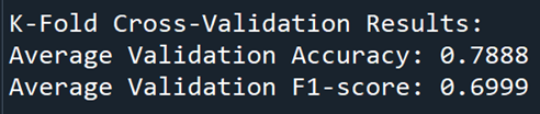
The results of the cross-validation, shown in the following picture, indicated an average accuracy of around 79% and an F1-score of approximately 70%. This suggested that our model performs fairly well, balancing precision and recall across the different classes.
Framework 2: SVM/FCNN
Since the average accuracy and F1-score are not high enough, this may be due to several factors. The language style and terminology used in FOMC documents might not fully align with FinBERT's training data. Additionally, FOMC documents often contain a large amount of neutral or ambiguous statements, which FinBERT might find difficult to interpret accurately. Furthermore, despite being based on the Transformer model, FinBERT may overlook the global context when processing long texts, resulting in less comprehensive sentiment analysis. Therefore, we decided to try another framework to redesign the model architecture.
Text Further Preprocessing
To further clean our text data, we used the Counter class to count word frequencies and set a threshold to eliminate less common terms. We filtered out "white noise" and applied part-of-speech tagging to gain insights into word usage. Named entity recognition helped us identify key entities, while n-grams captured common word pairings. These steps streamlined our data. The code we use is as follows:
# count frequency
word_freq = Counter(no_stops)
# set the threshold, word with a  frequency < threshold wil be removed
threshold = 4
# remove less frequent words
filtered_no_stops = [word for word in no_stops if word_freq[word] >= threshold]

#remove white noise
filtered_no_stops = [word for word in filtered_no_stops if word not in white_noise]

# Tagging
pos_tags = nltk.pos_tag(no_stops)

# Parsing
named_entities = nltk.chunk.ne_chunk(pos_tags)

# N-grams
ngs_stems = ngrams(stems, 2)
ngs_lemmas = ngrams(lemmas, 2)
Considering the existing code has already taken a long time to run (over twenty minutes), we decided to simplify and improve it. Firstly, we streamlined the text-cleaning function by removing the complex mapping table, making the character replacement process more straightforward. Secondly, the logic for data processing has also been optimized by introducing the process_text and process_documents functions, which encapsulate repetitive tasks and reduce redundancy. Furthermore, database operations have been refined by using helper functions like create_db_connection and insert_data, which simplified the connection and data insertion processes. As a result, the reprocessed code offers a clearer structure, making it easier to maintain and extend. Part of the modified code is as follows:
def process_documents(documents, new_list):
    for doc in documents:
        value = doc['text']
        words, stems, lemmas = process_text(value)
        new_list.append({
            'date': doc['date'],
            'type': doc['type'],
            'original': value,
            'tokenized': words,
            'stems': stems,
            'lemmas': lemmas
        })
Model: SVM
To utilize the original data, which has undergone extensive preprocessing, we turned to Support Vector Machine (SVM), a supervised learning model known for its effectiveness in classification tasks. SVM works by finding the optimal hyperplane that separates different classes in the feature space, making it particularly powerful for high-dimensional data.
We read all the text data and classified the federal rate data into different groups based on their values. Then, we employed the TF-IDF method to extract features from the text data. Subsequently, we split the dataset into training and testing sets, maintaining an 80% to 20% ratio.
During the model training process, we built the SVM model using the Scikit-learn library, selecting a simple linear kernel function. The code we use is as follows:
# Create and Train Support Vector Machine Classification Model
model = SVC(kernel='linear')  # Use linear kernel
model.fit(X_train, y_train)

# Make Predictions
y_pred = model.predict(X_test)

# Evaluate the Model
accuracy = accuracy_score(y_test, y_pred)
print(f"Accuracy: {accuracy:.2f}")
print("Reports:")
print(classification_report(y_test, y_pred))
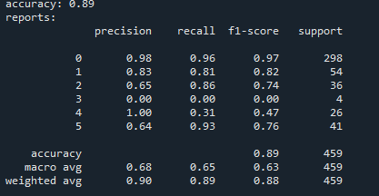
The results were excellent! For the target federal fund rate, when we limited the interval to 0.5%, the F1 score soared to 0.81. By relaxing the constraint to a 1% interval, the F1 score jumped to an impressive 0.89, as shown in the following picture. Meanwhile, for the effective federal fund rate, limiting the interval to 0.5% yielded an F1 score of 0.51, which increased to 0.62 when the constraint was relaxed to a 1% interval.
After careful considerations, we assume the reasons behind are that the target rate is directly influenced by the Federal Reserve's FOMC meetings, making it easier for the model to capture trends. In contrast, the effective federal fund rate (EFFR) is affected by various factors, including market liquidity and other macroeconomic variables, making it more difficult for the model to predict.
Additionally, we explored 5-fold cross-validation to further verify our model. Our evaluations revealed an average validation accuracy of 0.81 and an average validation F1-score of 0.80, both of which surpass the results achieved by the previous LSTM model.
Model: FCNN
However, recognizing the limitations of the simple linear kernel in our SVM model, we decided to enhance our approach by implementing a Fully Connected Neural Network (FCNN), which offers strong capabilities for nonlinear modeling.
We constructed a multilayer perceptron using Keras, employing the ReLU activation function for the hidden layers and the Softmax activation function for the output layer. The model was compiled with the Adam optimizer and categorical cross-entropy as the loss function. During the training process, we set the batch size to 32 and trained for 10 epochs. The code we use is as follows:
# Create the Neural Network Model
model = Sequential()
model.add(Dense(128, activation='relu', input_shape=(X_train.shape[1],)))  # Input layer
model.add(Dense(64, activation='relu'))  # Hidden layer
model.add(Dense(13, activation='softmax'))  # Output layer with 13 classes

# Compile the Model
model.compile(optimizer='adam', loss='categorical_crossentropy', metrics=['accuracy'])

# Train the Model
model.fit(X_train, y_train_cat, epochs=10, batch_size=32, validation_split=0.1)
The results were remarkable: the F1 score for the 0.5% interval improved to 0.92, while for the 1% interval, it reached an impressive 0.97, as shown in the picture.
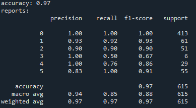
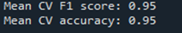
In terms of 5-fold cross-validation, the average validation accuracy and F1-score of 95%, as shown in the following picture, were the highest among all models. This demonstrates the strongest predictive capability our team has achieved through our research.
Conclusion
Our project explored two frameworks for predicting the federal funds rate using FOMC texts: the FinBERT + LSTM Neural Network and the SVM/FCNN approaches. The FinBERT + LSTM model achieved moderate accuracy (79%) and an F1-score (70%), but its performance may have been limited by the predominantly neutral sentiment scores generated by FinBERT and the complexity of FOMC language. In contrast, the SVM and FCNN models demonstrated superior performance, with the FCNN model achieving the highest average validation accuracy (95%) and F1-score (95%) for predicting the target federal funds rate.
In summary, we successfully accomplished our goals: analyzing Federal textual information to predict future rates using text analysis and NLP. We have trained an effective model that achieved an average validation accuracy of 95% and an F1-score of 95% for predicting the target federal funds rate using FOMC texts.
Thank you for reading our blog!