Clustering with Sentiment Analysis and Market Analysis (by Group "SFinx")

Text Processing

After scraping news data from Reuters, we perform text processing to clean and refine the content, preparing it for subsequent vectorization and clustering. Since the data collection phase already involved preprocessing and integration into a JSON file format (as mentioned in the first blog), this step primarily focuses on processing the article body to enhance its suitability for vectorization.

Key steps include:

1. Text Cleaning: Remove HTML tags, special characters, numbers, and normalize whitespace.

2. Tokenization & Filtering: Use regex-based tokenization to retain words with ≥2 letters, remove standard English stopwords(198) and custom stopwords (e.g., country names, dates, prepositions with 100+), and filter out long words (>10 letters).

3. Lemmatization: Perform context-aware lemmatization (e.g., running → run) using POS tagging to map words to their base forms accurately.

4. Data Integration: Process titles and bodies from JSON files, skip non-English or empty articles, and deduplicate based on titles.

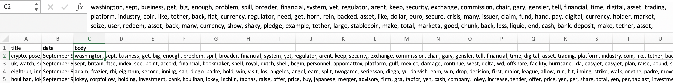
5. Format Conversion: Convert tokenized results into comma-separated strings and save as structured CSV.

Note: Since the code is too lengthy, please refer to our GitHub repository (Text_Preprocessing_V2) for the relevant implementation.

Challenges & Solutions

To further refine text quality, three targeted filtering steps were implemented to eliminate noise identified through iterative testing:

1. Residual Stop Words

Issue: Default stopword lists (NLTK) missed domain-specific terms (e.g., china, jan).

Solution: Expanded custom stopwords to include countries, dates, redundant terms (e.g., new, say), and prepositions—over 200 terms added.

stop_words = set(stopwords.words('english'))
custom_prepositions = {'above', 'across', 'after',...}
custom_stop_words = {'china', 'usa','say', 'jan',...}
stop_words.update(custom_prepositions)
stop_words.update(custom_stop_words)
tokens = [word for word in tokens if word not in stop_words]

2. Single-Letter Word Elimination

Issue: Despite initial tokenization rules (retaining ≥2-letter words), residual single-letter tokens like u appeared after lemmatization.

Solution: Added a final filter to enforce a minimum word length of 2 characters.

lemmatized_tokens = [word for word in lemmatized_tokens if len(word) >= 2]

3. Post-Lemmatization Specific Word Removal

Iteration Process:

V1: Removed common noisy words (e.g., licensing, right) early in preprocessing.

V2: Found residual terms like principle and new persisting after lemmatization. Revised the code to apply removal after lemmatization for completeness.

# Remove specific words (performed after lemmatization)
words_to_remove = {'licensing', 'right', 'thomson', 'trust', 'tabsuggested', 
                   'principle', 'open', 'new', 'standard', 'say', 'co', 'ltd'}
lemmatized_tokens = [word for word in lemmatized_tokens if word not in words_to_remove]

Key Design Choices

Multi-Stage Filtering: Progressive refinement via cleaning → stopword removal → length filtering → post-lemmatization pruning.

POS-Guided Lemmatization: Leveraged part-of-speech tagging for context-aware lemmatization, outperforming single-POS assumptions.

Lightweight Structuring: Output CSV retains only essential fields (title, date, body) to streamline downstream vectorization. Part of the CSV results is shown below:

Clustering

After text preprocessing, we employ TF-IDF vectorization to transform text into numerical representations, capturing key features for analysis. In the clustering phase, we utilize K-Means to identify distinct themes within financial news. This section outlines the code configuration and parameter tuning, ensuring efficient and insightful classification of financial news data.

Step 1: Word2Vec Model Training

To capture semantic relationships between words, we trained a Word2Vec model on the preprocessed text corpus. Key hyperparameters were systematically tuned to balance model performance and computational efficiency:

• vector_size(70–90): Controls the dimensionality of word embeddings. Higher values capture finer semantic nuances but increase complexity.
• window(8–10): Defines the context window size for training. Larger windows capture broader document-level themes.
• min_count(2–3): Filters out rare words to reduce noise while retaining domain-specific terms.
• N(10–20): To find the best number of important words that we should select from each document.

The goal of this part is to find the best parameters combination to find the meaningful words.

# The best parameters combination to train the Word2Vec Model
model = Word2Vec(sentences=test_data['content_tokens'], vector_size=80, window=9, min_count=2, workers=8)

Note: Since the code is too lengthy, please refer to our GitHub repository (find_parameter) for the relevant implementation.

Step 2: Clustering by K-means

Extracting Important Words with TF-IDF

After training the Word2Vec model, we used TF-IDF (Term Frequency-Inverse Document Frequency) to rank word importance within each document. We select the 20 most frequent words per article (based on inverse TF-IDF scores).

# Compute TF-IDF weights for all words in the dataset
corpus = test_data['content'].tolist()  
vectorizer = TfidfVectorizer()
tfidf_matrix = vectorizer.fit_transform(corpus)
word2tfidf = dict(zip(vectorizer.get_feature_names_out(), vectorizer.idf_))

# Identify high-frequency words per article
N = 20 # Number of top words per article, N also be found by the loop function
test_data['important_words'] = test_data['content_tokens'].apply(
    lambda tokens: sorted(
        set(tokens),  # Remove duplicates
        key=lambda x: word2tfidf.get(x, 0),  # Rank by TF-IDF score
        reverse=False  # Lower TF-IDF means higher frequency in this case
    )[:N]
)

Converting Text into Feature Vectors

Each document is represented as a weighted average of its word embeddings. This transforms unstructured text into numerical vectors suitable for clustering.

# Define a function to convert text to a weighted vector, use the word2vec model and the TF-IDF weights
def text_to_vector(text, model, word2tfidf):
    vectors = []
    weights = []
    for word in text:
        if word in model.wv:
            vectors.append(model.wv[word])
            weights.append(word2tfidf.get(word, 1.0))  # Default weight 1.0 if not in TF-IDF
    if not vectors:
        return np.zeros(model.vector_size)
    vectors = np.array(vectors)
    weights = np.array(weights) / sum(weights)  # Normalize weights
    return np.average(vectors, axis=0, weights=weights)

# Convert important words to vectors
test_data['vector'] = test_data['important_words'].apply(lambda x: text_to_vector(x, model, word2tfidf))

K-Means Clustering

We partitioned the documents into clusters using K-Means with num_clusters=2. Key steps included: 1. Scaling feature vectors to ensure equal contribution from all dimensions. 2. Running multiple initializations to avoid suboptimal local minima.

# Use the k-means algorithm to cluster the articles, split the data into two groups.
X = np.array(test_data['vector'].tolist())
num_clusters = 2  # Number of clusters
kmeans = KMeans(n_clusters=num_clusters, random_state=42)
labels = kmeans.fit_predict(X)
test_data['cluster_label'] = labels

Evaluating Clustering Performance

We use two metrics: 1. Silhouette Score: Measures how well clusters are separated. 2. Calinski-Harabasz Score: Evaluates the compactness of clusters. The best hyperparameters are chosen based on these scores.

# Evaluate clustering effect by calculating silhouette score and Calinski-Harabasz index
if 'cluster_label' in test_data and len(set(test_data['cluster_label'])) > 1:
    X = np.array(test_data['vector'].tolist())  # Assuming 'vector' is from the Word2Vec/KMeans pipeline
    labels = test_data['cluster_label'].values
    silhouette = silhouette_score(X, labels)
    ch_score = calinski_harabasz_score(X, labels)
    print(f"Silhouette Score: {silhouette:.3f}")
    print(f"Calinski-Harabasz Index: {ch_score:.3f}")
else:
    print("Unable to calculate clustering metrics: Either no 'cluster_label' column or fewer than 2 clusters.")

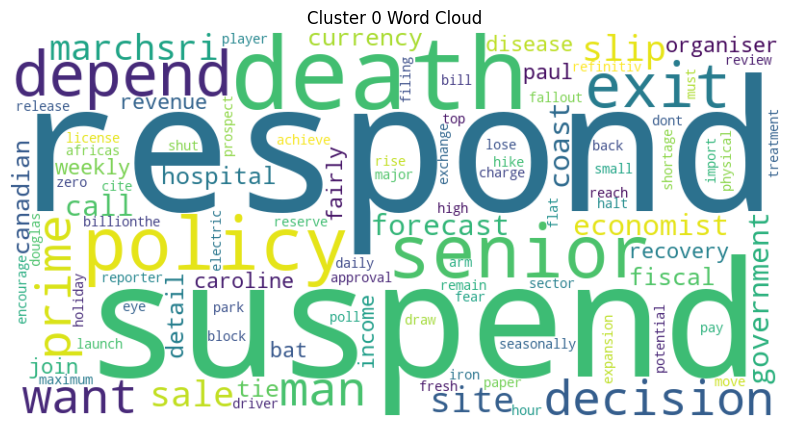
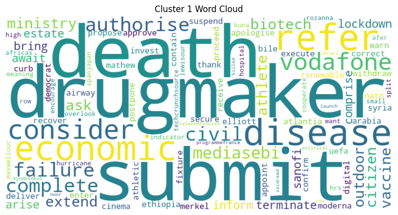
• WordCloud of Each Cluster: Generate the WordCloud for the high-frequency words in each cluster, based on data from January 2021 to August 2021, to visualize the details of each cluster.

Sentiment Analysis

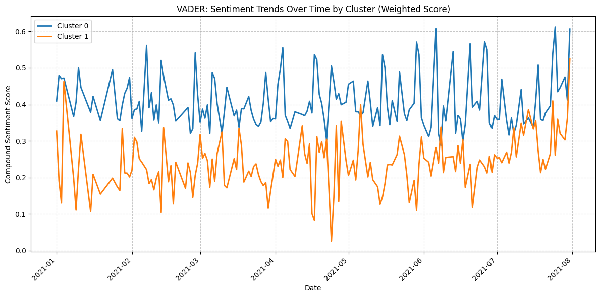
In this analysis, we used two sentiment analysis tools—VADER (general-purpose) and FinBERT (finance-specific)—to evaluate their effectiveness in extracting actionable insights from financial news clusters. Using a dataset of Reuters articles grouped into thematic clusters via K-Means, we measured sentiment polarity across clusters and dates.

Method 1: VADER for general sentiment analysis

VADER (Valence Aware Dictionary and sEntiment Reasoner) is a lexicon and rule-based sentiment analysis tool. It is specifically designed to analyze the sentiment of text in social media and other informal contexts. It works by looking at the words and phrases in the text, and then assigning sentiment scores based on a pre-defined dictionary of sentiment-laden words and a set of rules for combining those scores. Key advantages of VADER include its suitability for general text analysis and its speed and efficiency in processing large volumes of data.

Key Implementation Steps:

1. Date-Cluster Grouping: Group articles by publication date and predefined thematic clusters (e.g., "Monetary Policy" vs. "Market Risks").

2. TF-IDF Weighted Keywords: Extract top 20 keywords per article using inverse document frequency (IDF) to prioritize rare yet impactful terms. Calculate normalized TF-IDF weights for each keyword to reflect its contextual relevance.

3. Contextual Text Synthesis: Convert keyword lists into synthetic text snippets (e.g., ["inflation", "rate hike"] → "inflation rate hike").

4. Sentiment Scoring: Apply VADER’s rule-based polarity detection to each synthetic snippet. Compute weighted compound scores using:

   $$ \text{Weighted Score} = \sum (\text{Word Sentiment} \times \text{TF-IDF Weight}) $$

5. Temporal Aggregation: Calculate daily average sentiment scores per cluster, weighted by article frequency. Handle edge cases (e.g., empty articles) with zero-filling to maintain temporal continuity.

These code briefly introduces a framework of VADER and its application in sentiment analysis:

# Method 1: Use VADER to analyze sentiment of important words in each cluster
test_data['date'] = pd.to_datetime(test_data['date'])
grouped = test_data.groupby('date')

# Initialize VADER sentiment analyzer
analyzer = SentimentIntensityAnalyzer()
# Store daily sentiment results for each cluster
sentiment_results = []

for date, group in grouped:
    for cluster in range(num_clusters):
        cluster_data = group[group['cluster_label'] == cluster]
        sentiment_scores = []

        for important_words in cluster_data['important_words'].dropna():
            if isinstance(important_words, list):
                words = [word for word in important_words if word.lower() not in stop_words and word.isalpha() and len(word) > 2]
            else:
                continue  

            if not words:
                continue  

            # calculate word weights based on TF-IDF scores
            word_weights = np.array([word2tfidf.get(word, 1.0) for word in words])

            # Normalize word weights to sum to 1
            if word_weights.sum() == 0:
                word_weights = np.ones_like(word_weights) / len(word_weights)
            else:
                word_weights /= word_weights.sum()

            text = " ".join(words)

            try:
                sentiment = analyzer.polarity_scores(text)
                compound_score = sentiment['compound']
                positive_score = sentiment['pos']
                negative_score = sentiment['neg']
                neutral_score = sentiment['neu']

                # Calculate weighted sentiment scores
                weighted_sentiment = {
                    'compound': compound_score * word_weights.sum(),
                    'positive': positive_score * word_weights.sum(),
                    'negative': negative_score * word_weights.sum(),
                    'neutral': neutral_score * word_weights.sum()
                }

                sentiment_scores.append(weighted_sentiment)

            except Exception as e:
                print(f"Error processing text for date {date}, cluster {cluster}: {text[:50]}..., Error: {e}")
                continue


        # Calculate average sentiment scores
        if sentiment_scores:
            avg_sentiment = {
                'compound': np.average([s['compound'] for s in sentiment_scores], weights=[word_weights.sum()] * len(sentiment_scores)),
                'positive': np.average([s['positive'] for s in sentiment_scores], weights=[word_weights.sum()] * len(sentiment_scores)),
                'negative': np.average([s['negative'] for s in sentiment_scores], weights=[word_weights.sum()] * len(sentiment_scores)),
                'neutral': np.average([s['neutral'] for s in sentiment_scores], weights=[word_weights.sum()] * len(sentiment_scores))
            }

            sentiment_results.append({
                'date': date,
                'cluster': cluster,
                'sentiment_score': avg_sentiment['compound'],
                'positive_score': avg_sentiment['positive'],
                'negative_score': avg_sentiment['negative'],
                'neutral_score': avg_sentiment['neutral'],
                'num_samples': len(sentiment_scores)
            })
        else:
            sentiment_results.append({
                'date': date,
                'cluster': cluster,
                'sentiment_score': 0.0,
                'positive_score': 0.0,
                'negative_score': 0.0,
                'neutral_score': 0.0,
                'num_samples': 0
            })

# Create DataFrame from sentiment results
vade_sentiment_df = pd.DataFrame(sentiment_results)

# Print results
print("\nSentiment Analysis Results:")
vade_sentiment_df

Method 2: FinBERT for financial sentiment analysis

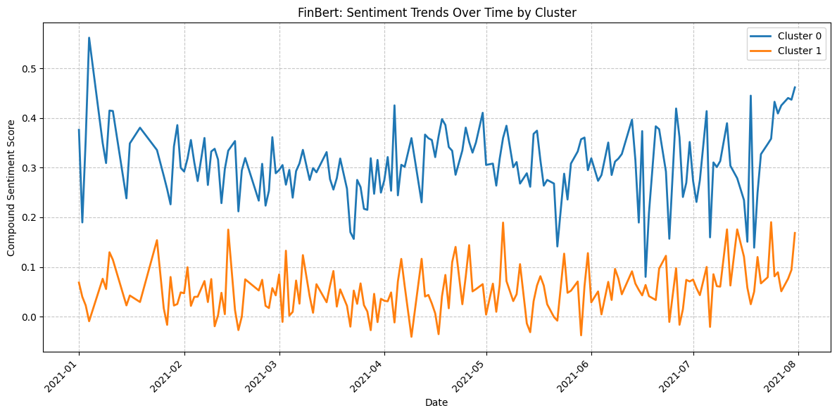
FinBERT is a sentiment analysis model based on the BERT (Bidirectional Encoder Representations from Transformers) architecture, specifically fine-tuned for financial text. It is used to analyze the sentiment of financial news, reports, earnings calls, and other financial-related text. It can understand the context and semantics of financial language, and classify the text into positive, negative, or neutral sentiment categories. Its key advantages include high accuracy in the financial domain, strong contextual understanding, and robust generalization ability across various financial texts.

Using HuggingFace’s AutoTokenizer and AutoModelForSequenceClassification, we load the pre-trained weights of the yiyanghkust/finbert-tone model, which is explicitly fine-tuned to recognize financial jargon (e.g., "quantitative easing," "bear market") and contextual nuances in economic narratives.

The following are the code for Model Initialization:

# Method 2: Use FinBERT for sentiment analysis
# Load FinBERT model and tokenizer
model_name = "yiyanghkust/finbert-tone"  # FinBERT model fine-tuned for financial sentiment
tokenizer = AutoTokenizer.from_pretrained(model_name)
model = AutoModelForSequenceClassification.from_pretrained(model_name)

Result

Each date - cluster pair is associated with an average sentiment score. A comparison of the results obtained from VADER and FinBERT reveals that Cluster 0 has a higher proportion of positive scores than Cluster 1. Moreover, the results from FinBERT appear to be more accurate or of better quality than those from VADER.

• Results from VADER (Based on Data from January 2021 to August 2021)

• Result from FinBert (Based on Data from January 2021 to August 2021)

Processing of Market Data

Fetching Financial Data

To fulfil the objectives of our project regarding trading strategies, we have selected some indices and commonly used sector ETFs as examples:

• Obtain historical data (Open/High/Low/Close/Adj Close/Volume) from Yahoo Finance.

tickers = [
    '^GSPC',    # S&P 500
    '^IXIC',    # NASDAQ
    'SPY',      # SPY (S&P 500 ETF)
    'QQQ',      # QQQ (NASDAQ ETF)
    'XLK',      # Tech Sector ETF
    'XLF',      # Financials ETF
    'XLE',      # Energy ETF
    '^VIX',     # Market Volatility (VIX)"
]

Symbol = ['S&P500', 'NASDAQ', 'SPY', 'QQQ', 'Tech_ETF', 'Financials_ETF', 'Energy_ETF', 'VIX']

# Define date range (e.g., past 5 years)
start_date = '2019-01-01'
end_date = '2023-12-31'

# Fetch data
data = yf.download(
    tickers=tickers,
    start=start_date,
    end=end_date,
    # Optional: Adjust granularity (default is daily)
    interval='1d',  # '1d', '1wk', '1mo'
    # Fetch adjusted close prices to account for splits/dividends
    auto_adjust=False
)

• Extract "Adj Close" for all tickers.

adj_close = data['Adj Close'].dropna()
adj_close.columns = Symbol

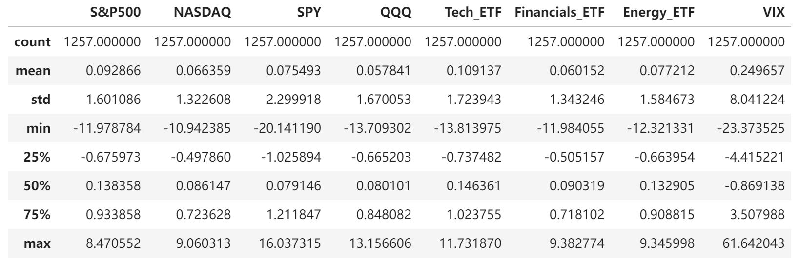
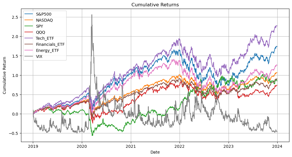
• Calculate daily percentage returns and cumulative returns(assuming reinvestment).

daily_returns = adj_close.pct_change() * 100  # Returns in percentage
daily_returns = daily_returns.dropna()  # Remove first row (NaN)

# Calculate cumulative returns (assuming reinvestment)
cumulative_returns = (1 + daily_returns / 100).cumprod() - 1

Generating csv file

daily_returns.to_csv('daily_returns.csv')
adj_close.to_csv('adjusted_close_prices.csv')

Visualization

• Plot Cumulative Returns

• Plot Correlation Heatmap

• Descriptive Statistics of Daily Returns