During the presentation, due to time limitations, we could not fully share how the sentiment analysis and the tuning of the machine learning model were done. Therefore, we would like to provide a more detailed description of these two items in this blog post.
Note: If you wish to run the sample code in this post, make sure to install and import the required packages.
from graphviz import Digraph
import numpy as np
import pandas as pd
import matplotlib.pyplot as plt
from NewsSentiment import TargetSentimentClassifier
tsc = TargetSentimentClassifier()
from nltk.tokenize import sent_tokenize #covered in our content, but not used in the code
from textblob import TextBlob
from statistics import mean
import re
import optuna
from sklearn.model_selection import StratifiedKFold
from xgboost import XGBClassifier
from sklearn.metrics import accuracy_score
1. Sentiment Analysis
Our analysis consists of mainly two parts: + Computing the average sentiment from articles for every day in range + Computing the lagged effect of the average sentiments for every day in range
1.1. Average Sentiment from articles on the same day
Use this code to reproduce the graph locally:
dot = Digraph()
# Create nodes
dot.node('R', 'Raw text data on a centain day')
dot.node('F', 'Filtered data')
dot.node('T', 'Tokenized data')
dot.node('BG', 'Background')
dot.node('TAR', 'Target')
dot.node('BG_P', 'Background Polarity')
dot.node('TAR_S', 'Target Sentiment')
dot.node('TAR_P', 'Target Polarity')
dot.node('TOT_P', 'Total Polarity of the day')
dot.node('AVG_P', 'Average Polarity of articles on that day')
# Add edges
dot.edge('R', 'F', label='\tFilter out articles containing\n\t \'NVDA\', \'NVIDIA\' or \'Nvidia\'')
dot.edge('F', 'T', label='\tSentence Tokenization')
dot.edge('T', 'BG', label='\tSentences without \n\t \'NVDA\', \'NVIDIA\', \'Nvidia\'')
dot.edge('T', 'TAR', label='\tSentences with \n\t \'NVDA\', \'NVIDIA\', \'Nvidia\'')
dot.edge('BG', 'BG_P', label='\tAverage Polarity Score \nusing "TextBlob"')
dot.edge('TAR', 'TAR_S', label='\t Probabilities of Positivity \n\tof each sentence using "NewsSentiment"')
dot.edge('TAR_S', 'TAR_P', label='\t Conversion from Probabilities to Polarity')
dot.edge('BG_P', 'TOT_P', label='\t Weight=0.2')
dot.edge('TAR_P', 'TOT_P', label='\t Weight=0.8')
dot.edge('TOT_P', 'AVG_P', label='\t Divide by the number of articles in \"Filtered data\"')
dot.edge('F', 'AVG_P', label='\t no. of articles')
dot
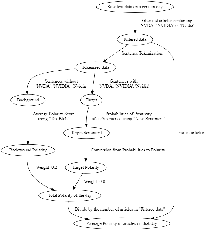
Our sentiment analysis for this part is illustrated in the graph.
1. Filtering
Basically, after web scraping, we ordered all the articles by date. From this, we filter out those that contain NVDA, NVIDIA or Nvidia (target) only, and discard all other irrelevant articles.
2. Sentence Tokenization
After that, we would perform sentence tokenization for each article using the nltk package. Then we can separate the sentences that mentioned the target and those that did not.
At this step, we would also check if the sentences contain weird symbols/hyperlinks or other things that may affect the sentiment analysis. If there is, we would remove them by means of string manipulation or regex.
3. Sentiment for sentences not mentioning the target
For those sentences that did not mention the target, we use Textblob to obtain an overall polarity of those sentences. Since the article itself contains the target, these sentences are still considered useful, but we will assign a lower weight of 0.2 to this polarity, and we will combine this with another score later.
4. Sentiment for sentences mentioning the target
For those sentences that mentioned the target, we instead use NewsSentiment to analyze the inferred positivity of the sentence to the target, as this package can better identify the positivity towards a specific noun in the sentence. The output of the NewsSentiment is actually a dictionary with 3 elements, which are positive, negative, and neutral.
For example, if the sentence is "I love NLP." and the target is set as "NLP", the output may be something like: {'positive': 0.9, 'negative': 0.05, 'neutral': 0.05}.
From this, we assign a weight of (1,0,-1) to positive, neutral and negative respectively, and then we can obtain the polarity of the sentence towards the target in general. For our example, the output would be 0.9*1+0.05*0+0.05*-1=0.85
Using this method, we can obtain the score for every sentence that mentioned our target, then we average out the sentinments, and assign a weight of 0.8 to it.
5. Combining sentiments for the day
Using the results from Step 3 & 4, we can then add up scores from every articles published on the same day, and divide by the number of articles. This gives us the average polarity of articles on that day.
Code Extract of daily sentiment analysis
Here, we provide an extract of our code for analyzing articles.
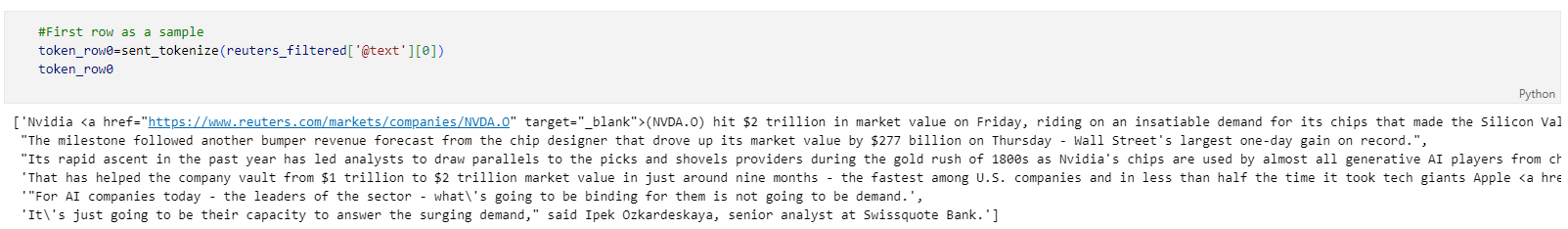
1. Function for removing links
In the data of Reuters, the tokenized sentences consist of html tags which represent hyperlinks. We then defined our own function to handle them in one go.
def remove_link(tokens):
    for i in range(len(tokens)):
        links=re.findall("<a href.*?>\([A-Z]{4}.O\)", tokens[i])
        if links:
            for link in links:
                tokens[i]=tokens[i].replace(" "+link, "")
    return tokens
remove_link(token_row0)

2. Function for handling the sentiment calculation
def tokensentiment(tokens):
    withoutN=[] #sentences without Nvidia using Textblob
    withN=[] #sentences with Nvidia using NewsSentiment
    for i in tokens:
        if i.find("Nvidia")==-1 and i.find("NVDA")==-1 and i.find("NVIDIA")==-1:
            withoutN.append(TextBlob(i).sentiment[0])
        else:
            mod_text=i.replace("Nvidia's", "Nvidia").replace("NVDA", "Nvidia").replace("NVIDIA", "Nvidia")
            s=mod_text.split("Nvidia")
            try:
                sentiment = tsc.infer_from_text(s[0],"Nvidia", s[1])
                pos,neg=0,0
                for j in sentiment:
                    if j['class_label']=="positive":
                        pos=j['class_prob']
                    if j['class_label']=="negative":
                        neg=j['class_prob']
                withN.append(pos-neg)
            except: withN.append(TextBlob(mod_text).sentiment[0]) #Use Textblob for edge cases
    if withoutN and withN:
        return mean(withoutN)*0.2+mean(withN)*0.8
    elif not withN: return mean(withoutN)
    else:    return mean(withN)
This code handles Steps 3 & 4 of the below workflow.
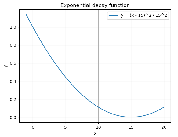
1.2. Lagged effect for the Sentiment scores
Since news would have a lagged effect on the stock. We then introduce an exponential weight decay approach to compute the final sentiment score of each day. We designed each new article would fade out in 15 days, a plot of the function is as below:
x = np.linspace(-1, 20, 100)

# Define the function
y = ((x - 15) ** 2) / (15 ** 2)
plt.plot(x, y, label='y = (x - 15)^2 / 15^2')

# Add labels and title
plt.title('Exponential decay function')
plt.xlabel('x')
plt.ylabel('y')

plt.grid(True)
plt.legend()
plt.show()
Using this decay function, we can then compute the effect of articles across multiple days. In the following example, we denote the Average Polarity of articles on day X as PX and the function of weight decay as f(Day after news is published)\ [Note: the first day is day 0].
Let's say on Day 1, we have some articles which give us P1, then on Day 2 we have P2, and on Day 3 we have P3.
Use this code to reproduct the graph locally:
#Compute the final sentiment score of a day
FS = Digraph()
#Create nodes
FS.node('P1', 'P1')
FS.node('P2', 'P2')
FS.node('P3', 'P3')
FS.node('D1', 'Score of Day 1')
FS.node('D2_t', 'Sum of weighted scores\n\t of Day 2')
FS.node('D2', 'Score of Day 2')
FS.node('D3_t', 'Sum of weighted scores\n\t of Day 3')
FS.node('D3', 'Score of Day 3')
#Computation of Scores
FS.edge('P1', 'D1', label='\tP1*f(0)')
FS.edge('P1', 'D2_t', label='\tP1*f(1)')
FS.edge('P2', 'D2_t', label='\tP2*f(0)')
FS.edge('D2_t', 'D2', label='\tDivide by num. of articles=2')
FS.edge('P1', 'D3_t', label='\tP1*f(2)')
FS.edge('P2', 'D3_t', label='\tP2*f(1)')
FS.edge('P3', 'D3_t', label='\tP3*f(0)')
FS.edge('D3_t', 'D3', label='\tDivide by num. of articles=3')

FS
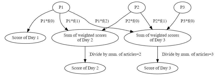
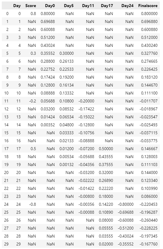
To better illustrate, lets consider a simple example:
#define the weights
weights=[round(((i - 15) ** 2) / (15 ** 2),4) for i in range(15)]

#Sample Scores
score_sample=pd.DataFrame({
"Day":[i for i in range(30)],
"Score":[np.nan]*30})

#add 5 sentinment scores
score_sample.iloc[0,1]=0.8
score_sample.iloc[5,1]=0.3
score_sample.iloc[11,1]=-0.2
score_sample.iloc[17,1]=0.5
score_sample.iloc[24,1]=-0.8
score_sample[:10]
We defined a function to append new columns for every sentiment value. And the new column would consist of all weighted decay sentiments related to that sentiment value. Then, we compute the mean across each row and get the final score that we would use in the time-series analysis and machine-learning models.
def appendnewcol(row,sentiment):
    newcol=[np.nan]*(row-0)+list(sentiment*np.array(weights))+[np.nan]*(len(score_sample)-row-15)
    if len(newcol)>len(score_sample):
        newcol=newcol[:len(score_sample)]
    score_sample[f'Day{row}']=newcol
scores=score_sample['Score'].tolist()
for i in range(len(scores)):
    if not np.isnan(scores[i]):
        appendnewcol(i,scores[i])
score_sample['Finalscore']=score_sample.iloc[:,2:].mean(axis=1, skipna=True)
Note: In the real data, there might be some days that have no articles published. In this case, we would interpolate the date values to ensure the date column is continuous.
sen.index = pd.to_datetime(sen['Date'])
sen=sen.resample('D').asfreq() #sample interpolation that we used in the real data
2. Automatic Hyperparameter Optimization
During the presentation, we illustrated the result of the XGBoost model, but it is well-known that such a decision tree model would require extensive hyperparameter tuning to achieve good results. Therefore, we would like to share the method that we used, which is a package named Optuna (https://github.com/optuna/optuna) for automatic hyperparameter optimization.
Here is a sample code for a binary classifier training with cross-validation, assuming the X y data are loaded in as data frames.
RETRAIN_MODEL = False #change to True to retrain
def objective(trial):
    # Define hyperparameters to tune
    param = {
        'objective':'binary:logistic',
        'learning_rate': trial.suggest_float('learning_rate', 0.005, 0.5),
        'n_estimators': trial.suggest_int('n_estimators',50,1000),
        'reg_alpha': trial.suggest_float('reg_alpha', 1e-8, 10.0,log=True),
        'reg_lambda': trial.suggest_float('reg_lambda', 1e-8, 10.0,log=True),
        'max_depth': trial.suggest_int('max_depth', 3, 20),
        'colsample_bytree': trial.suggest_float('colsample_bytree', 0.3, 1.0),
        'subsample': trial.suggest_float('subsample', 0.5, 1.0),
        'min_child_weight': trial.suggest_int('min_child_weight', 1, 5),
        #'device' : "cuda", #use gpu as necessary
        'tree_method':"hist"
    }

    cv = StratifiedKFold(n_splits=10, shuffle=True, random_state=42)
    auc_scores = []

    for train_idx, valid_idx in cv.split(X, y):

        X_train_fold, X_valid_fold = X.iloc[train_idx], X.iloc[valid_idx]
        y_train_fold, y_valid_fold = y.iloc[train_idx], y.iloc[valid_idx]

        model = XGBClassifier(**param)
        model.fit(X_train_fold, y_train_fold)
        preds = model.predict(X_valid_fold)
        acc=accuracy_score(y_valid_fold, preds)
        auc_scores.append(acc)

    return np.mean(auc_scores)

study = optuna.create_study(direction='maximize',study_name = "xgb_model_training")

if RETRAIN_MODEL:
    study.optimize(objective, n_trials=100)  # Adjust the number of trials as necessary

    print(f"Best trial average AUC: {study.best_value:.4f}")
    for key, value in study.best_params.items():
        print(f"{key}: {value}")
Using this package, we can automatically collect the optimized hypermeters instead of performing grid search/alternate optimization manually.