As students who wish to pursue a career in markets, we aim to identify curve trade opportunities on U.S. Treasuries with NLP. To forecast the short end of the curve (i.e. 2Y Treasury yields), we aim to analyze sentiments extracted from FOMC minutes given the short end is very sensitive to Fed Fund rate adjustments. Whereas for the long end (i.e. 10Y-30Y Treasury yields), the further out we go on the yield curve, the less casual impact there is using just sentiment to explain the curve. Hence, we plan to monitor macroeconomic indicators such as demand and supply of bonds; inflation expectations, inflation expectations being the second order impact of CPI/ NFP/ PCE. Using forecasted yield spread derived from FOMC meeting sentiments and macro datas, we hope to predict yield spreads to come up with curve trade strategies to make profits.

Text Retrieval

Step 1: Locate FOMC article in Press Release site and Copy Texts

To retrieve FOMC minutes, we used Selenium to loop through every article on the Press Release page looking for headlines that contained "FOMC statement".

Once the program locates the headline, it will click into the link and copy all the texts. However, the automation of text scraping may induce some elements to experience delays in loading, causing the Element Not Visible Exception. To prevent the exception, we adopted explicit wait command, which tells the Webdriver to wait for a maximum of 10 seconds for an element matching the given criteria to be found. Below is the programme that visits the FOMC article and extracts meeting minutes.

for i in range(len(fomcLink)):
    link = WebDriverWait(driver, 10).until(
    EC.presence_of_all_elements_located((By.PARTIAL_LINK_TEXT, "FOMC statement")))[i] 
    print(link.get_attribute('href'))

    driver.execute_script("arguments[0].click()", link)
    link_text = WebDriverWait(driver, 10).until(
    EC.presence_of_element_located((By.ID, "article")))
    print(link_text.text)

    driver.back()

Step 2: Visit Next Page on Press Release Site

After all statements have been extracted from the page, the programme would visit the next Press Release page and repeat this process. This is done by telling Webdriver to click the "Next" button on the page bar at the end of the site.

It was found that sometimes the Webdriver cannot perform this action since the element is not visible on the page. In order to locate the element, one would need to scroll to the bottom of the site. Here, we relied on JavaScript Executor to execute the command, which would help to capture the element.

 next = WebDriverWait(driver, 20).until(
    EC.presence_of_element_located((By.LINK_TEXT, "Next")))
driver.execute_script("arguments[0].click()", next)

Step 3: Convert Extracted Texts into Tabular Form

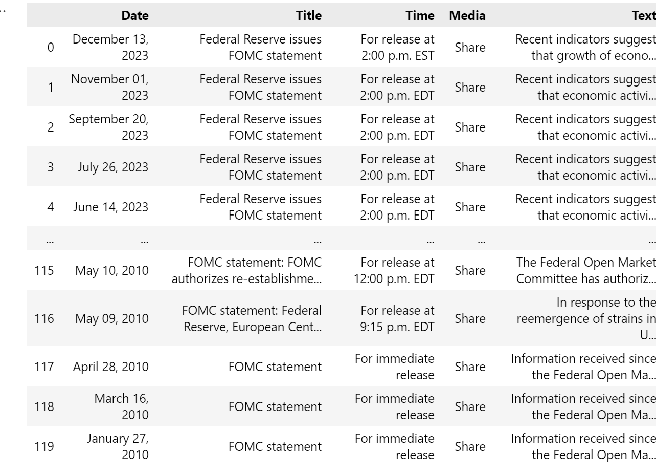
We observed the extracted minutes were already well-formatted, since the meeting time and meeting minutes were separated into different paragraphs.

To convert extracted minutes into Tabular form indexed by time, all that remained was to split the texts by a new line (i.e. \n) and format them into lists.

def writeText(text):
    splitted = text.split('\n', 4)

In the end, using Pandas library the text data are being exported as excel file for further analysis.

Text Preprocessing

Having extracted the minutes from the FOMC website, we initiated the text preprocessing phase to standardize the content and eliminate any extraneous elements. This meticulous process aims to enhance the quality of the text, ensuring optimal conditions for subsequent sentiment analysis.

Step 1: Read Data from CSV File

Our first step involves extracting data from the CSV file.

The code we use is as follows:

# read csv file
import pandas as pd
df = pd.read_csv('FOMC_text.csv')

Step 2: Remove Unrelated Paragraphs

Upon importing the data, our task is to examine the content structure and eliminate irrelevant paragraphs. In the context of our FOMC example, we identified paragraphs pertaining to voting members, contact methods and issue dates that were irrelevant to our analysis and consequently removed them. It is noteworthy that these paragraphs shared a common starting phrase, prompting us to address this consistent pattern during our data refinement process.

The code we use is as follows:

# Removal of unrelated paragraph
import re
def Removal_paragraph(text):
    text = re.sub(r'Voting for the monetary policy action.*','',text)
    text = re.sub(r'For media inquiries.*','',text)
    text = re.sub(r'Implementation Note issued.*','',text)
    return text
df['text_related'] = df['Text'].apply(lambda x: Removal_paragraph(x))

Step 3: Convert to Lowercase

To further enhance uniformity and facilitate consistent analysis, we proceeded to convert all text entries to lowercase.

The code we use is as follows:

# Convert to lowercase
df['lowercase_text'] = df['text_clean'].str.lower()

Step 4: Lemmatization & POS Tagging

For optimal efficiency in transforming words into their meaningful base forms, we employ lemmatization. To enhance accuracy, we leverage Part-of-Speech (POS) tagging to annotate the grammatical categories of each word. This strategic use of POS tagging ensures that lemmatization is executed with improved precision, contributing to more accurate and meaningful results.

The code we use is as follows:

# Lemmatization & POS Tagging
from nltk import pos_tag
from nltk.corpus import wordnet
from nltk.stem import WordNetLemmatizer
lemmatizer = WordNetLemmatizer()
wordnet_map = {"N":wordnet.NOUN, "V": wordnet.VERB,"J": \
               wordnet.ADJ, "R": wordnet.ADV}
def lemmatize_words(text):
    # find pos tags
    pos_text = pos_tag(text.split())
    return " ".join([lemmatizer.lemmatize(word,\
    wordnet_map.get(pos[0], wordnet.NOUN)) for word, pos in pos_text])
df['lemmatized_text'] = df['lowercase_text'].apply(lambda x: lemmatize_words(x))

Step 5: Remove Punctuations within the Sentence

Following the standardization of the text, our next step involved the removal of punctuation within the sentences. However, we made a deliberate choice to retain essential punctuation marks such as ".", "?", and "!" to preserve the sentence structure. This decision was driven by the necessity to maintain the integrity of the text in sentence format, as we require sentiment scores for each individual sentence.

The code we use is as follows:

# Removal of Punctuations within the sentence
def remove_punctuations(text):
    punctuations = "\"#$%&'()*+-/:;<=>@[\]^_`{|}~"
    return text.translate(str.maketrans('', '', punctuations))
df['clean_text_1'] = df['lemmatized_text'].apply(lambda x: remove_punctuations(x))

Step 6: Remove Stopwords

Commonly occurring words like articles, prepositions, and conjunctions, known as stopwords, are abundant but contribute minimally to extracting the essence of text. Following the elimination of punctuation within the sentences, we deliberately exclude stopwords. This strategic step allows us to concentrate on the more meaningful and content-rich words, thereby enhancing the flow of analysis and optimizing overall efficiency.

The code we use is as follows:

# Removal of stopwords
from nltk.corpus import stopwords
STOPWORDS = set(stopwords.words('english'))
def remove_stopwords(text):
    return " ".join([word for word in text.split() if word not in STOPWORDS])
df['clean_text_2'] = df['clean_text_1'].apply(lambda x: remove_stopwords(x))

Step 7: Remove Numbers and Extra Spaces

In the conclusive phase of our text preprocessing process, we systematically eliminate numerical digits and extraneous spaces. This step aims to enhance the relevance and meaningfulness of the text specifically for sentiment analysis, as numbers and extra spaces hold little significance in this context.

The code we use is as follows:

# Removal of Punctuations within the Sentence
import re
def remove_spl_chars(text):
    text = re.sub('[\d]', ' ', text)
    text = re.sub('\s+', ' ', text)
    return text
df['clean_text_3'] = df['clean_text_2'].apply(lambda x: remove_spl_chars(x))

Data Preprocessing Results

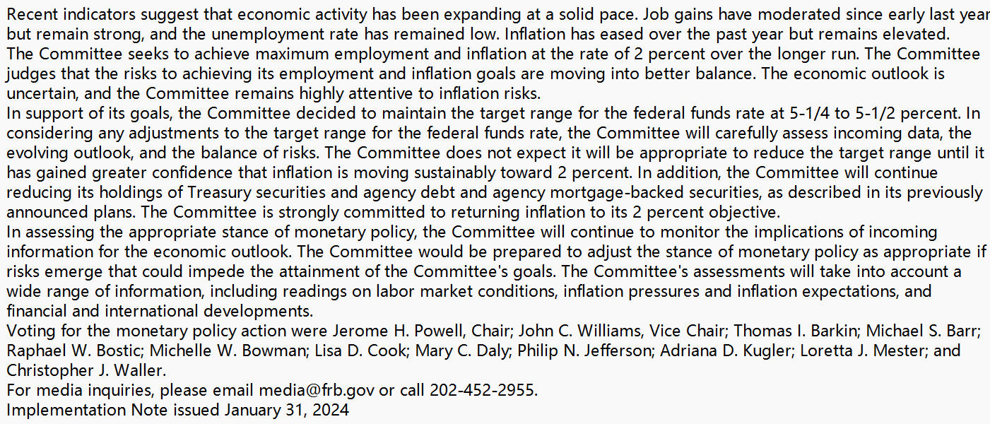
We will utilize a minute from the FOMC website as an illustrative example to showcase the outcomes. Through this, we anticipate witnessing a marked enhancement in relevance and clarity, particularly conducive to more accurate sentiment analysis.

Original text

Clean text

Sentiment Score

To construct an appropriate measurement that reflects the sentimental information behind FOMC minutes, and then makes predictions about the interest rate fluctuation indirectly, we plan to try 2 optional methods - CNN(Convolutional Neural Networks) and TextBlob, both of which can return to a float number showing the sentimental tendency of the Federal Reserve on interest rate policy.

We will share our insights and provide corresponding examples in followings.

Option 1: CNN

Convolutional Neural Networks (CNNs) are a class of deep neural networks commonly used for analyzing visual imagery. They are designed to automatically and adaptively learn spatial hierarchies of features from the input data. However, instead of its traditional application in image recognition, we leverage its ability to learn some difficult structures embedded in input data more accurately, so that we can quantitatively learn how possible the Federal Reserve will increase the policy rate next period by 'deep learning' FOMC texts and their sentimental structures.

Typically, the CNN algorithm mainly consists of following steps:

1. Word Embeddings: Convert each word in the sentence into its word embedding representation, which captures semantic and contextual information.

2. Padding: Since sentences may have different lengths, padding can be used to make all input sequences of equal length.

3. Convolutional Layers: These layers apply convolution operations to the input, using filters that detect specific features in the input data. The filters slide over the input data to capture patterns.

4. Pooling Layers: Pooling layers down-sample the feature maps generated by the convolutional layers, reducing the spatial dimensions of the data while retaining important information.

5. Activation Functions: Non-linear activation functions like ReLU (Rectified Linear Unit) introduce non-linearities to the network, enabling it to learn complex patterns in the data.

6. Fully Connected Layers: These layers connect every neuron in one layer to every neuron in the next layer, helping to classify the features extracted by earlier layers.

These code briefly introduces a framework of CNN and its application in sentiment analysis:

import numpy as np
from keras.models import Sequential
from keras.layers import Embedding, Conv1D, GlobalMaxPooling1D, Dense

# Example data
sentences = ["I loved the NLP!", "The result was terrible.", "The method was average."]
labels = [1, 0, 0]  # 1 for positive sentiment, 0 for negative sentiment

# Preprocess the data
vocab_size = 10000  # Size of the vocabulary
max_length = 20  # Maximum length of input sentences

# Tokenize the sentences and pad them to a fixed length
tokenizer = Tokenizer(num_words=vocab_size)
tokenizer.fit_on_texts(sentences)
sequences = tokenizer.texts_to_sequences(sentences)
padded_sequences = pad_sequences(sequences, maxlen=max_length)

# Create the CNN model
embedding_dim = 100  # Dimension of word embeddings
num_filters = 128  # Number of filters in convolutional layer

model = Sequential()
model.add(Embedding(vocab_size, embedding_dim, input_length=max_length))
model.add(Conv1D(num_filters, 5, activation='relu'))
model.add(GlobalMaxPooling1D())
model.add(Dense(1, activation='sigmoid'))

# Compile the model
model.compile(optimizer='adam', loss='binary_crossentropy', metrics=['accuracy'])

# Train the model
model.fit(padded_sequences, np.array(labels), epochs=10, batch_size=32, validation_split=0.2)

# Make predictions
test_sentences = ["The movie was great!", "I didn't enjoy it."]
test_sequences = tokenizer.texts_to_sequences(test_sentences)
padded_test_sequences = pad_sequences(test_sequences, maxlen=max_length)
predictions = model.predict(padded_test_sequences)

# Print the predictions
for i, sentence in enumerate(test_sentences):
    sentiment = "positive" if predictions[i] > 0.5 else "negative"
    print(f"Sentence: {sentence}")
    print(f"Sentiment: {sentiment}")

In this example, we use the Keras library to build a CNN model for sentiment analysis. We tokenize the input sentences, pad them to a fixed length, and then define the model architecture using the Embedding, Conv1D, GlobalMaxPooling1D, and Dense layers. We compile the model with an optimizer, loss function, and metrics, and then train it on the labeled data. Finally, we make predictions on new test sentences and print the predicted sentiment.

Method 2: TextBlob

Another option to explore sentimental tendency is TextBlob, a prepared module in Python. TextBlob originally holds a sentimental semantic classifier, categorizing 'sentimental words' into different labeled groups. When measuring the probability that a certain sentence conveys positive/negative attitude, TextBlob turns to 'Naive Bayes Classifier' , which assigns input data the predicted state corresponding to the maximum conditional probability given current state.

Here is the specification of 'Naive Bayes Classifier':

1. Let 𝒙={𝒂_𝟏, 𝒂_𝟐, 𝒂_𝟑,…,𝒂_𝒏} be a item to be classified, where 𝒂_𝒊 represents a characteristic of 𝒙.

2. Denote our sentiment labels as 𝒔={𝒔_𝟏, 𝒔_𝟐, 𝒔_𝟑,…,𝒔_𝒎}.

3. Calculate the conditional probabilities and find the largest one:

   𝑷(𝒔_𝒌│𝒙)=𝒎𝒂𝒙{𝑷(𝒔_𝟏│𝒙),𝑷(𝒔_𝟐│𝒙),…, 𝑷(𝒔_𝒎│𝒙)}

   then we categorize the item 𝒙 into sentiment label 𝒔_𝒌.

To practically apply TextBlob module, we can just import it and call the 'sentiment.polarity' function. The following are the demo codes:

from textblob import TextBlob

# Simple function to output sentiment score
def get_sentiment_score(text):
    blob = TextBlob(text)
    sentiment_score = blob.sentiment.polarity
    return sentiment_score

# Example usage
text = "The weather tends to be terrible tomorrow"
sentiment_score = get_sentiment_score(text)
print(sentiment_score)   

Accuracy and Training Set

In order to enhance the accuracy of our model when making decisions on relatively long texts, we calculate the mean of TextBlob sentiment score of each sentence in an article, so that the final result becomes more comprehensive and smoother.

The code we use is as follows:

sentiment_list = []  

# text_list contains all articles to be analyzed.
for text in text_list:
    sub_sentiment_list = []
    for sentence in text:
        blob = TextBlob(sentence)
        sentiment_score = blob.sentiment.polarity
        sub_sentiment_list.append(sentiment_score)
    sentiment_list.append(sub_sentiment_list.mean())

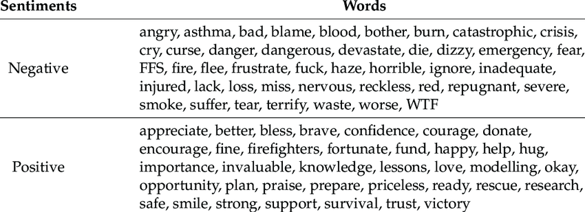
On the other hand, default sentiment classifier may not fit enough in the context of interest rate policies. The prediction system will perform better if we can insert our own training set that maps the Federal Reserve’s statements on interest rate policies to several custom labels.

Traditional Sentimental Words Classification

A Word Cloud relating to Interest Rate Policy