By Group "Five Sigma"

This blog aims to explore curve trade opportunities in U.S. Treasuries by analyzing sentiments extracted from Federal Open Market Committee (FOMC) minutes. In the first part, we meticulously refined our sentiment score calculation process to address encountered challenges building upon the methodology outlined in our previous blog. After experimenting with three different methods for calculating sentiment scores, we derived results suitable for regression analysis. In the second part, we conducted regression analyses separately for the short and long ends of the yield curve. We elucidate the rationale behind selecting independent variables and detail how we accounted for them in our regression models using the Ordinary Least Squares methodology. Additionally, we explore other variables influencing 10-year yields and conclude that sentiment scores alone may not adequately explain fluctuations in long-term yields. Overall, our findings suggest that while sentiment analysis proves valuable for forecasting the short end of the yield curve, additional factors beyond sentiment are crucial for comprehensively understanding and predicting movements in long-term Treasury yields.

Part I：Sentiment Score Calculation

To construct an appropriate measurement that reflects the sentiment information behind FOMC minutes, and then makes predictions about the interest rate fluctuation indirectly, we tried 3 methods - Keras, TextBlob and Pysentiment2 to compute polarity scores showing the sentiment tendency of the Federal Reserve on interest rate policy.

1. Procedure

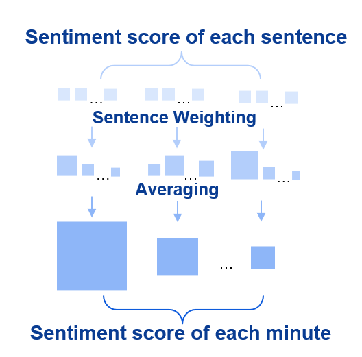
The following is a flowchart of our attempt to calculate the sentiment score for each FOMC minute. First, we clean the text content, then split each minute into sentences, and call a module to calculate the sentiment score for each sentence. Afterward, we weight and average the scores to obtain the sentiment score for each minute. Each step of this process will be further discussed in the following sections, where we will detail the specific implementation steps required for the code.

2. Methods to Compute Sentiment Scores of Sentences

2.1 Keras

Introduction

Keras is a Python library for building and training deep learning models, offering advanced neural network APIs. It supports various types of models, including Convolutional Neural Networks (CNNs) and Recurrent Neural Networks (RNNs). Keras stands out for its flexibility and scalability, enabling users to construct complex neural network architectures and train them efficiently on different hardware platforms. Widely applied in processing diverse data like images, audio, and text, Keras plays a crucial role in the field of deep learning. Leveraging Keras' adeptness at capturing intricate structures in input data, we can perform quantitative analysis of FOMC minutes and their underlying sentiment structures.

Process

(1) Preparation In the initial phase, we assemble a comprehensive dataset comprising text samples paired with their corresponding sentiment labels. For instance, a sample might be labeled as positive or negative based on its sentiment. This dataset is then split into distinct subsets for training, validation, and testing. Then we load the pretrained Word2Vec model and use it to obtain the embedding matrix for words. This embedding matrix will be utilized in the Embedding layer of the model to map words from the text data to vector representations. By mapping words to the corresponding word vectors in the Word2Vec model, we can obtain semantic information for words and use them as inputs to the neural network model.

# Assemble the dataset comprising text samples and their corresponding sentiment labels
import numpy as np
from gensim.models import KeyedVectors

# Load pretrained Word2Vec embeddings
def load_pretrained_word2vec_embeddings(file_path):
    word2vec_model = KeyedVectors.load_word2vec_format(file_path, binary=True)
    embedding_matrix = np.zeros((vocab_size, embedding_dim))
    for word, i in tokenizer.word_index.items():
        if word in word2vec_model:
            embedding_matrix[i] = word2vec_model[word]
    return embedding_matrix

# Replace 'file_path' with the actual path to your Word2Vec model file
word2vec_file_path = 'path/to/word2vec_model.bin'
embedding_matrix = load_pretrained_word2vec_embeddings(word2vec_file_path)

#Sample
sentences = ["I loved the NLP!", "The result was terrible.", "The method was average."]
labels = [1, 0, 0]  # 1 for positive sentiment, 0 for negative sentiment

(2) Text Processing Text processing involves removing noise, special characters, and stop words from the text to ensure the data is clean and ready for analysis. The detailed process can be found in the Text Preprocessing section of our previous blog. Then, we convert the textual tokens into numerical representations. Initially, we read the cleaned text data from a CSV file and store it in a DataFrame. The text is tokenized, breaking it down into individual words or tokens, and parameters such as vocabulary size and maximum sentence length are defined. Using the Tokenizer class from the Keras library, we convert the text tokens into numerical sequences, with each word represented by a unique integer based on its frequency in the corpus. These sequences are padded to a fixed length to ensure uniform input size, crucial for neural network processing.

# Convert the textual tokens into numerical representations
from tensorflow.keras.preprocessing.text import Tokenizer
from keras.preprocessing.sequence import pad_sequences

# Tokenize the sentences and pad them to a fixed length
vocab_size = 10000  # Size of the vocabulary
max_length = 20  # Maximum length of input sentences

tokenizer = Tokenizer(num_words=vocab_size)
tokenizer.fit_on_texts(sentences)
sequences = tokenizer.texts_to_sequences(sentences)
padded_sequences = pad_sequences(sequences, maxlen=max_length)

(3) Model Building In this stage, we construct the model architecture by adding layers such as embedding layers, LSTM/GRU layers, or convolutional layers. We experiment with different architectures, layer types, and hyperparameters to identify the optimal configuration for our model.

# Construct the CNN model architecture
from keras.models import Sequential
from keras.layers import Embedding, Conv1D, GlobalMaxPooling1D, Dense

# Load pretrained word embeddings (Word2Vec)
embedding_dim = 100  # Dimension of word embeddings
# Load pretrained word embeddings from file and update the embedding matrix
embedding_matrix = np.random.rand(vocab_size, embedding_dim)
# Number of filters in convolutional layer
num_filters = 128

# Create the CNN model with pretrained word embeddings
model = Sequential()
model.add(Embedding(vocab_size, embedding_dim, weights=[embedding_matrix], input_length=max_length, trainable=False))
model.add(Conv1D(num_filters, 5, activation='relu'))
model.add(GlobalMaxPooling1D())
model.add(Dense(1, activation='sigmoid'))

(4) Model Training The model is trained on the training dataset using the fit() function. During training, we fine-tune parameters such as batch size, number of epochs, and learning rate to enhance model performance. We closely monitor the training process and evaluate the performance of model on the validation set to ensure its effectiveness.

# Compile and train the model
model.compile(optimizer='adam', loss='binary_crossentropy', metrics=['accuracy'])
model.fit(padded_sequences, np.array(labels), epochs=10, batch_size=32, validation_split=0.2)

(5) Model Prediction Once the model is trained, we preprocess new data in the same manner as the training data. The preprocessed data is then fed into the model to obtain predictions. This process involves importing relevant modules and functions, tokenizing the text to form a sequence, calling the LSTM model function, and adjusting parameters for optimal performance. Finally, we input test texts to make predictions, leveraging the predictive capabilities of our trained model.

# Preprocess new data and make predictions
test_sentences = ["The movie was great!", "I didn't enjoy it."]
test_sequences = tokenizer.texts_to_sequences(test_sentences)
padded_test_sequences = pad_sequences(test_sequences, maxlen=max_length)
predictions = model.predict(padded_test_sequences)

# Print the results
for i, sentence in enumerate(test_sentences):
    sentiment = "positive" if predictions[i] > 0.5 else "negative"
    print(f"Sentence: {sentence}")
    print(f"Sentiment: {sentiment}")

2.2. TextBlob

Introduction

TextBlob is a Python library for natural language processing (NLP) tasks, offering simple yet powerful tools for tasks such as text processing, sentiment analysis, part-of-speech tagging, and more. Its strength lies in its user-friendly API and extensive functionality, enabling users to quickly perform text processing and sentiment analysis without needing to delve into complex NLP techniques. It is suitable for handling general text data, such as social media comments, news articles, and more. TextBlob leverages an internal emotion lexicon(Pattern Library is used in our analysis) to compute polarity scores, which gauge the positivity of text on a scale from -1 (very negative) to 1 (very positive).

Process

We start by importing the necessary modules and defining a function called get_sentence_sentiment_scores. This function accepts a list of texts as input and calculates sentiment scores for each sentence within the texts. Within the function, we iterate through each text, splitting it into sentences using the sentences method in TextBlob. For each sentence, sentiment scores are computed using the sentiment.polarity attribute in TextBlob. These scores, along with the count of sentences in each text, are collected into two lists: sentence_sentiment_scores and sentence_counts, respectively. Then, the function returns these lists, providing sentiment scores for each sentence and the number of sentences in each text.

from textblob import TextBlob
import pandas as pd

# Calculate the sentiment scores and the number of sentences for each text
def get_sentence_sentiment_scores(text_list):
    sentence_sentiment_scores = []
    sentence_counts = []
    for text in text_list:
        # Split the text into sentences
        text_with_periods = text.replace('.', '. ')
        print(text_with_periods)
        sentences = TextBlob(text_with_periods).sentences
        print(sentences)
        sentence_counts.append(len(sentences))
        # Calculate sentiment scores for each sentence and add them to the list
        for sentence in sentences:
            sentiment_score = sentence.sentiment.polarity
            sentence_sentiment_scores.append(sentiment_score)
    return sentence_sentiment_scores, sentence_counts

# Get the sentiment scores for each sentence and the count of sentences for each text
sentence_scores, sentence_counts = get_sentence_sentiment_scores(text_list)

Next, we tally the sentiment scores of all sentences in each text, computing their average by dividing the total by the number of sentences. These average scores, paired with their corresponding text identifiers, are structured into a DataFrame. Finally, we save this DataFrame as a CSV file named average_sentiment_scores.csv. This file offers insights into the prevailing sentiment trend by providing average sentiment scores for each unit of analysis.

avg_sentiment_scores = []
start_index = 0
for count in sentence_counts:
    end_index = start_index + count
    avg_score = sum(sentence_scores[start_index:end_index]) / count
    avg_sentiment_scores.append(avg_score)
    start_index = end_index

result_df = pd.DataFrame({'Text': range(1, len(avg_sentiment_scores) + 1),'Average_Sentiment_Score': avg_sentiment_scores})
result_df.to_csv('average_sentiment_scores.csv', index=False)

Unexpected Outcomes and Potential Reasons

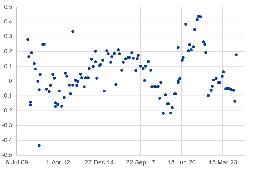
The scatter plot below illustrates the sentiment scores for each FOMC minute, which were computed using the TextBlob method.

The unexpected outcomes prompt us a deeper exploration of potential factors influencing these results. Two primary considerations emerged:

(1) Textual Characteristics: Linguistic biases inherent in speeches manifested in skewed results favoring positive values. This phenomenon underscores the need for a nuanced understanding of language nuances and biases. Linguistic biases inherent in speeches manifested in skewed results favoring positive values. This phenomenon underscores the need for a nuanced understanding of language nuances and biases.

(2) Pattern Library Suitability: TextBlob method relies solely on pre-defined sentiment scores without considering the nuances of financial language or the specific context of FOMC minutes. The inherent limitations of models of the Pattern library in capturing the intricacies of specific language styles observed in minutes. These models may inadequately capture the complexities of financial language, thereby compromising the accuracy of sentiment analysis outcomes.

2.3. Pysentiment2

Introduction

Pysentiment2 is a library for sentiment analysis in a dictionary framework with two dictionaries provided, namely, Harvard IV-4 and Loughran and McDonald Financial Sentiment Dictionaries. We chose the Loughran and McDonald Financial Sentiment Dictionaries which are sentiment dictionaries tailored for financial sentiment analysis, furnishing invaluable insights into the prevalence of positive and negative words, alongside the polarity and subjectivity inherent in the text.We believe that by invoking a sentiment lexicon specialize in the financial text domain, the results will be improved.

Process

The following code demonstrates how we invoke PySentiment2 and utilize the Loughran and McDonald Financial Sentiment Dictionaries to compute sentiment scores. We first import the LM class from the PySentiment2 module. We then initialize an instance of the LM class. Next, we define a function called calculate_sentiment_score which takes a text input and computes the sentiment score using the Loughran and McDonald Financial Sentiment Dictionaries provided by PySentiment2. Finally, we demonstrate how to use this function to calculate the sentiment score for text.

# Import the LM class from the Pysentiment2 module
import pysentiment2 as ps
lm = ps.LM()
# Take a text input and compute the sentiment score using the LM Dictionaries
def fin_sentiment(sentence):
    tokens = lm.tokenize(sentence)
    score = lm.get_score(tokens)
    return score

# Calculate the sentiment scores and the number of sentences for each text
def get_sentence_sentiment_scores(text_list):
    for text in text_list:
        # Split the text into sentences
        text_with_periods = text.replace('.', '. ')
        sentences = TextBlob(text_with_periods).sentences
        # Count number of sentences in one FOMC statement
        sentence_counts.append(len(sentences))
        # Calculate sentiment scores for each sentence and add them to the list
        for sentence in sentences:
            sentiment_score = fin_sentiment(str(sentence))
            sentence_length.append(len(sentence))

3. Sentence Weighting Methods

3.1.Key Words Weighting

Our first attempt at sentence weighting involved identifying key words within each sentence and applying a weight proportional to the number of keywords present. However, since keywords were found in most sentences, this method was limited in effectively capturing nuanced sentiment variations.

3.2.Sentence Length Weighting

This method entailed multiplying sentiment score of each sentence by its respective length, reflecting the notion that longer sentences may encapsulate richer semantic content. We finally adopted the sentence length weighted approach, applying it in the first step of our sentiment analysis procedure. By aggregating the weighted sentiment scores and computing their average, we derived the final sentiment score for each minute.

# Calculate sentiment scores for each sentence and add them to the list
for sentence in sentences:
    sentiment_score = fin_sentiment(str(sentence))
    sentence_length.append(len(sentence))
# Locate poliarty score from dictionary, then calculate sentiment using length of sentiment as weight
    sentiment_score = len(sentence)*(list(sentiment_score.values())[2])
    sentence_sentiment_scores.append(sentiment_score)

4. Results

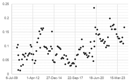
The scatter plot below illustrates the sentiment scores for each FOMC minute, which were computed using the Pysentiment method. In the following regression analysis, we will use the sentiment score as an independent variable.

Part II：Regression Analysis

Short-end

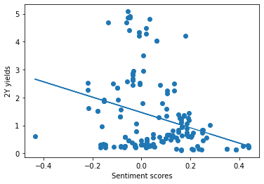
We conducted an analysis to assess the relationship between sentiment scores, obtained via PySentiment2, and 2-year Treasury yields, with the timing of FOMC meetings serving as a reference point on the horizontal axis. The graphical representation revealed an inverse relationship between the two variables, supporting our initial hypothesis that sentiment scores could be indicative of future movements in 2-year Treasury yields.

Prior to conducting regression analysis, we standardized the frequency of sentiment score data to align with other datasets. This adjustment was necessary because FOMC meetings, which occur eight times annually, are not evenly distributed throughout the year. To achieve uniformity, we recalibrated the dates of FOMC meetings to the end of the corresponding month; for instance, a meeting in mid-December would be represented as December 31st. This allowed us to bring forward sentiment scores to months that do not have FOMC meetings, facilitating our regression analysis.

Using the matplotlib library for visualization, we observed a tentative inverse relationship between sentiment scores and 2-year yields. However, the regression's explanatory power was relatively weak, with an R-squared value of approximately 0.09.

Attempts to enhance model accuracy through regression on lagged variables resulted in a decrease in R-squared. We tried incorporating the Personal Consumption Expenditures (PCE) into our multivariate regression. We found that while sentiment scores and 2-year yields maintained an inverse relationship, PCE exhibited a positive relationship with 2-year yields.

Nonetheless, the improvement in our model's R-squared was minimal, indicating that further refinement and exploration of other data manipulation techniques might be required to achieve more robust results.

Based on short-end regression analysis, we plotted two graphs：

(1) Scatter Plot of Sentiment Scores vs. 2Y Yields (No Lag): The first graph is a scatter plot with sentiment scores on the x-axis and 2-year yields on the y-axis. It also fits a linear regression line to the scatter plot. The polyfit function fits a polynomial of degree 1 (a straight line) to the data points, and poly1d constructs the polynomial equation. The coefficient of determination (r2_score) is printed, which indicates how well the linear regression line fits the data points.

(2) 3D Scatter Plot of Sentiment Scores, PCE YoY, and 2Y Yields (No Lag): The second graph is a 3D scatter plot with sentiment scores and PCE YoY on the x and y axes, respectively, and 2-year yields on the z-axis. It also fits a regression plane to the scatter plot using least squares regression (np.linalg.lstsq). The coefficients of the regression plane are used to create a mesh grid (x_plane, y_plane, z_plane), and then the regression plane is plotted on the 3D scatter plot.

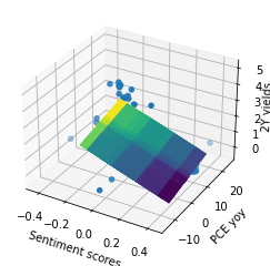
By visualizing the relationships among these variables, the graph helps us assess whether there are any discernible patterns or correlations.

The code used for plotting is as follows.

from sklearn.linear_model import LinearRegression
import matplotlib.pyplot as plt
import pandas as pd
import numpy as np
from sklearn.metrics import r2_score
from mpl_toolkits.mplot3d import Axes3D

df = pd.read_excel('Pysentiment vs. FFR.xlsx', 'Input')

# Extracting variables from excel
TwoYear_yields = df['2Y_Yields']
Sentiment_score = df['Score_(EOM)']
PCE_yoy = df['PCE']

# No lag (sentiment vs. 2y yields)
plt.scatter(Sentiment_score, TwoYear_yields)
z = np.polyfit(Sentiment_score, TwoYear_yields, 1)
p = np.poly1d(z)
plt.xlabel('Sentiment scores')
plt.ylabel('2Y yields')
plt.plot(Sentiment_score,p(Sentiment_score))
print(r2_score(TwoYear_yields, p(Sentiment_score)))

# correlation_matrix = np.corrcoef(Sentiment_score, TwoYear_yields)
# correlation_xy = correlation_matrix[0,1]
# print(correlation_xy**2)

# No lag (sentiment & pce vs. 2y yields)
fig = plt.figure()
ax = fig.add_subplot(111, projection='3d')
ax.scatter(Sentiment_score, PCE_yoy, TwoYear_yields)

# Fit a plane using np.linalg.lstsq
A = np.vstack([Sentiment_score,PCE_yoy,np.ones_like(Sentiment_score)]).T
plane_coef, _, _, _ = np.linalg.lstsq(A, TwoYear_yields, rcond=None)

# Create a meshgrid for the plane
x_plane, y_plane = np.meshgrid(Sentiment_score, PCE_yoy)
z_plane = plane_coef[0] * x_plane + plane_coef[1] * y_plane + plane_coef[2]

# Add the regression plane
surfacePlot = ax.plot_surface(x_plane, y_plane, z_plane, cmap='viridis', \
            alpha = 0.7, linewidth=0, antialiased=True, shade=True)
#fig.colorbar(surfacePlot, orientation='horizontal')

# fig.colorbar(ax.plot_surface(x_plane, y_plane, z_plane), shrink=0.5, aspect=5) 

# Add labels and title
ax.set_xlabel('Sentiment scores')
ax.set_ylabel('PCE yoy')
ax.set_zlabel('2Y yields')
ax.zaxis.labelpad = -3.5
#plt.title('Multivariate Regression')
plt.show()

# Compute r^2 for multivariate regression
model = LinearRegression()
X, y = df[['Score_(EOM)', 'PCE']], df['2Y_Yields']
model.fit(X ,y)
print(model.score(X, y))

Long-End

To understand whether the average sentiment score can predict long-end movements, we employed Ordinary Least Squares (OLS) multivariate regressions by regressing the y-variable (10-year) on x-variables, namely PCE, S&P 500, and the average sentiment score. Our first model’s x-variables included the Personal Consumption Expenditures (PCE) year-over-year (YoY) change, the S&P 500 YoY change, and the average sentiment score. In contrast, the second model excluded the sentiment score to examine its effect in combination with the aforementioned factors.

Our first model yielded an R-square of 0.13; whereas the second model yielded an R-square of 0.044, meaning that without the sentiment score, PCE YoY and S&P 500 YoY can only explain 4.4% of the variance in the 10-year yield. The choice of PCE as a variable was motivated by its significant role in driving approximately 70% of U.S. GDP.

The Federal Reserve's preference for PCE over the Consumer Price Index (CPI), coupled with a stronger statistical correlation between PCE and the 10-year yield compared to CPI, reinforced its inclusion in our analysis.

The inclusion of the S&P 500 index was based on the observed interplay between stock market performance and bond yields, which, despite varying across different macroeconomic conditions, often sees investors turn to U.S. Treasury bonds as a "safe haven" during times of stock market downturns.

Our decision to measure variables in terms of YoY changes rather than absolute levels was driven by the OLS methodologies. Changes, represented by YoY, provide more informational value than levels; OLS tries to fit a line of best fit, and fitting it to any point more would mean compromising the level of fitting to other points; when doing YoY, it 1) tracks the direction of travel of the line which contains more informational values; 2) gives less noise than month-over-month (MOM); 3) is a way of normalizing variables.

However, our findings indicate that the average sentiment score alone does not sufficiently explain the movements of the 10-year yield. This conclusion underscores the complexity of factors influencing long-term interest rates and highlights the significance of other factors affecting the long end. One such factor is the volume of Treasury issuance; another is the term premium on the 10-year yield. Using the Fisher equation, TP = nominal interest rate - real interest rate - inflation rate, is a crucial element in understanding yield dynamics.