By Group "Financial Language Insights"
This blog aims to recap the journey of the "Reddit Trader" project. Our ultimate goal is to use the power of Reddit sentiment analysis to predict stock price movements. Throughout the Data Processing and Binary Classifier Training process, encountering challenges was to be expected. While we have devised solutions for certain hurdles, there are still lingering issues that we are actively addressing. Join us in this blog as we reflect on our journey, share valuable insights, and strive to assist fellow students who may encounter similar difficulties.
Problem 1: Database
We initially utilized the Python package PRAW to scrape Reddit posts. However, a limitation became apparent since it could only collect a maximum of 1000 items regardless of parameter adjustments. In practice, we could only retrieve 250 posts due to additional restrictions. Consequently, we were unable to acquire a substantial amount of Reddit data using this package.
Solution: We addressed this issue by using PRAW to scrape only the latest data within the year 2024 ensuring that our dataset captured the most up-to-date data. For historical data before 2024, we leveraged Pushshift Dumps which provided us with third-party crawled data. By merging these two methods, we obtain rich training and testing datasets. In light of the intricate nature of the code within Pushshift Dumps, we will only present a comprehensive guide on utilizing the PRAW package here:
import praw
import pandas as pd
from datetime import datetime

# PRAW setup and authentication
reddit = praw.Reddit(client_id='your_client_id',
                     client_secret='your_client_secret',
                     user_agent='your_user_agent')

# Function to capture recent posts using PRAW
def recent_search(reddit, subreddit_name, query, limit):
    subreddit = reddit.subreddit(subreddit_name)

    topics = {'score': [],
              'date': [],
              'title': [],
              'userid': [],
              'link': [],
              'body': [],
             }

    for submission in subreddit.search(query=query, sort='top', limit=limit, time_filter='year'):
        topics['score'].append(submission.score)
        topics['date'].append(submission.created)
        topics['title'].append(submission.title)
        topics['userid'].append(submission.id)
        topics['link'].append(submission.url)
        topics['body'].append(submission.selftext)

    df = pd.DataFrame(topics)
    df['date'] = df['date'].apply(lambda x: datetime.strftime(datetime.fromtimestamp(x), '%Y-%m-%d'))
    return df

# Parameters
subreddit_name = 'wallstreetbets'  # The subreddit to search
query = 'APPLE'  # The query to search for in post titles or bodies
limit = 1000  # Maximum number of posts to retrieve

# Capture recent posts using PRAW
recent_posts = recent_search(reddit, subreddit_name, query, limit)

# Print the captured posts
print(recent_posts)
Problem 2: Sentiment Analysis of Comments
This issue was brought about by Problem One. Concerned about the potential insufficiency of post quantity obtained through PRAW (before we find "Pushshift Dumps" as a solution), we explored the idea of simultaneously scraping comments and discovered PRAW’s robust capability to retrieve comments. However, a challenge arose due to the hierarchical comment system on Reddit, where comments are organized in a tree-like structure. This posed a problem for sentiment analysis because it could not accurately determine whether an emotional comment was directed towards the post itself or the mentioned stock. For example, if the post is "NVIDIA is terrible" and the comment is "You are terribly wrong," the sentiment score of this comment would be negative, despite it is actually supporting NVIDIA, that is, a positive attitude towards the stock!
from nltk.sentiment import SentimentIntensityAnalyzer

# Sentiment analysis function
def sentiment_analysis(text):
    sia = SentimentIntensityAnalyzer()
    sentiment_scores = sia.polarity_scores(text)
    sentiment_score = sentiment_scores['compound']
    return sentiment_score

# Example sentiment analysis
post_text = "NVIDIA is terrible"
comment_text = "You are terribly wrong"

post_sentiment = sentiment_analysis(post_text)
comment_sentiment = sentiment_analysis(comment_text)

print("Post Sentiment:", post_sentiment)
print("Comment Sentiment:", comment_sentiment)
Here is the expected return, indicating that comments originally expressing extremely positive sentiment towards stocks have been assessed as highly negative:
Post Sentiment: -0.4767
Comment Sentiment: -0.6249
Solution: Considering that many sentiment analysis packages are unable to handle such scenarios effectively, we made the decision to forgo analyzing comments and focus solely on analyzing the main posts.
Problem 3: Sentiment Analysis Package
Initially, we relied on the NLTK Vader for sentiment analysis of Reddit posts. However, upon conducting our inspection, we discovered that it often yielded inaccurate results. For instance, an evident negative sentiment expressed in a post such as " Nvda is a huge bubble right now." was misclassified as positive due to the positive connotation of "bubble" outside the financial domain:
Original Post: Nvda is a huge bubble right now.
Compound Score: 0.6996
Sentiment Label: positive
Solution: We have decided to combine three sentiment analysis packages, namely NLTK, Afinn, and TextBlob. Despite their limitations in handling complex language patterns, the integration of these packages reduced the occurrence of errors, resulting in minimal impact on the overall results. Through our inspection, we have found that the majority of the analyses produce accurate outcomes. To further enhance the accuracy of sentiment analysis in financial texts, it is crucial to allocate sufficient time and resources for exploring deep learning methods.
Problem 4: Score = 0
The sentiment score data contains many zeroes. One scenario is when sentiment analysis fails to determine a clear emotional inclination for posts on a specific day, resulting in a neutral state. However, a more severe issue arises when there is a lack of data due to the absence of crawled data for popular posts on that day, leading to data gaps that can negatively impact subsequent training.
Solution: To address this problem, we employ interpolation using two methods. The first method is k-nearest neighbors (KNN):
KNN is a simple and non-parametric machine learning algorithm that predicts the label or value of a new input based on the majority class or average value of its K closest training examples.
from sklearn.impute import KNNImputer

def consolidate(company, symbol, weekend, neighbor):
    # Aggregate sentiment of posts by post date
    sentiment_df = pd.read_csv("../Sentiment/" + company + "_Sentiment.csv")
    sentiment_df_1 = sentiment_df[['date','compound','pos','neg','neu']].groupby(['date']).mean()

    # Merge sentiment data with stock data
    stock_df = pd.read_csv("../stock_data/" + symbol + ".csv")
    stock_df = stock_df[stock_df['tic'] == 'GOOG']
    if weekend == False:
        consolidated = stock_df.merge(sentiment_df_1, how='left', left_on='datadate', right_on='date')
    else:
        # Interpolate imaginary weekend stock price
        stock_df['datadate'] = pd.to_datetime(stock_df['datadate'])
        start_date = stock_df['datadate'].min()
        stock_df.set_index('datadate', inplace=True)
        stock_df = stock_df.resample('D', origin=start_date).ffill()
        stock_df = stock_df.reindex(stock_df.index.strftime("%Y-%m-%d")).reset_index()
        consolidated = stock_df.merge(sentiment_df_1, how='left', left_on='datadate', right_on='date')
        consolidated[['prccd','prchd','prcld','prcod']] = consolidated[['prccd','prchd','prcld','prcod']].interpolate(method='linear', limit_direction='forward', axis=0)

    # K-nearest neighbor imputation
    consolidated[['index','compound','pos','neg','neu']] = KNNImputer(n_neighbors=neighbor).fit_transform(consolidated[['compound','pos','neg','neu']].reset_index())
    consolidated = consolidated.drop(['gvkey','tic','iid','index'], axis=1)

    return consolidated
The second method is momentum interpolation, referred to as "consolidate_pre." It involves extending the trend of sentiment scores from the preceding days to fill in the missing data. Overall, KNN performs better than "consolidate_pre," but it has a limitation. It may utilize data from subsequent periods that were unknown at the time. We can only assume that KNN can simulate such trends through machine learning.
import pandas as pd

def consolidate_pre(company, symbol, neighbor):
    # Aggregate sentiment of posts by post date
    sentiment_df = pd.read_csv("../Sentiment/" + company + "_Sentiment.csv")
    stock_df = pd.read_csv("../stock_data/" + symbol + ".csv")

    # Remove all the data with ticker 'GOOGL'
    if symbol == 'GOOG':
        stock_df = stock_df[stock_df['tic'] == 'GOOG']

    #interpolate imaginary weekend stock price
    stock_df['datadate'] = pd.to_datetime(stock_df['datadate'])
    start_date = stock_df['datadate'].min()
    stock_df.set_index('datadate', inplace=True)
    stock_df = stock_df.resample('D', origin=start_date).ffill()
    stock_df = stock_df.reindex(stock_df.index.strftime("%Y-%m-%d")).reset_index()

    # Merge sentiment data with stock data
    merged_df = stock_df.merge(sentiment_df, how='left', left_on='datadate', right_on='date')

    # drop date and rename datadate to date
    merged_df = merged_df.drop(['date'], axis=1)
    merged_df = merged_df.rename(columns={'datadate': 'date'})

    # reserve date, prccd, sentiment_score
    merged_df = merged_df[['date', 'prcod', 'prccd', 'sentiment_score_NLTK', 'sentiment_score_Afinn', 'sentiment_score_Textblob']]

    #interpolate missing stock price
    merged_df[['prccd']] = merged_df[['prccd']].interpolate(method='linear', limit_direction='forward', axis=0)
    merged_df[['prcod']] = merged_df[['prcod']].interpolate(method='linear', limit_direction='forward', axis=0)

    # set NaN in sentiment_score to the pre value
    merged_df['sentiment_score_NLTK'] = merged_df['sentiment_score_NLTK'].fillna(method='ffill')
    merged_df['sentiment_score_Afinn'] = merged_df['sentiment_score_Afinn'].fillna(method='ffill')
    merged_df['sentiment_score_Textblob'] = merged_df['sentiment_score_Textblob'].fillna(method='ffill')

    # drop the NaN in sentiment_score
    merged_df = merged_df.dropna(subset=['sentiment_score_NLTK'])

    merged_df.to_csv("../Consolidated/" + company + "_pre.csv")
Problem 5: Algorithm Selection
During the Binary Classifier Training, we initially explored four relatively simple algorithms: K-Nearest Neighbors (KNN), Logistic Regression, Support Vector Machine (SVM), and Naive Bayes:
from sklearn.model_selection import train_test_split
from sklearn.neighbors import KNeighborsClassifier
from sklearn.model_selection import cross_val_score
from sklearn.linear_model import LogisticRegression
from sklearn.svm import SVC
from sklearn.naive_bayes import MultinomialNB
from sklearn.preprocessing import MinMaxScaler

def Learning(train_df, test_df, factor):
    val_results = collections.defaultdict(int)

    #Set training set and test set
    x=np.array(train_df[['sentiment_score_'+factor]])
    y=np.array(train_df['buy_or_sell'])
    x_train, x_test, y_train, y_test = train_test_split(x, y, test_size = 0.1, random_state = 0)

    #K-Nearest-Neighbors
    neigh = KNeighborsClassifier(n_neighbors=5)
    neigh.fit(x_train, y_train)
    neigh.score( x_test, y_test)

    neigh_cv = cross_val_score(neigh, x_train, y_train, cv=10)
    val_results['K-Nearest-Neighbors'] = neigh_cv.mean()


    #Logistic Regression
    logreg = LogisticRegression(random_state=66)
    logreg.fit(x_train, y_train)
    logreg.score( x_test, y_test)

    logreg_cv = cross_val_score(logreg, x_train, y_train, cv=10)
    val_results['Logistic Regression'] = logreg_cv.mean()

    #Support Vector Machines
    svm_linear = SVC( kernel = 'sigmoid')
    svm_linear.fit(x_train, y_train)
    svm_linear.score(x_test, y_test)

    svm_linear_cv = cross_val_score(svm_linear, x_train, y_train, cv=10)
    val_results['Support Vector Machines'] = svm_linear_cv.mean()

    #Naive Bayes
    scaler = MinMaxScaler()
    X_minmax = scaler.fit_transform(x_train)

    mnb = MultinomialNB()

    mnb_cv = cross_val_score(mnb, X_minmax, y_train, cv=10) # uscaled data accuracy same;  6588046192259676
    val_results['Naive Bayes'] = mnb_cv.mean()
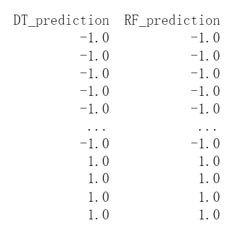
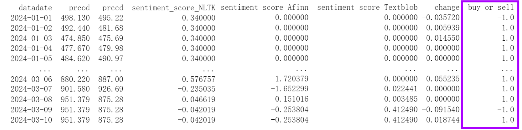
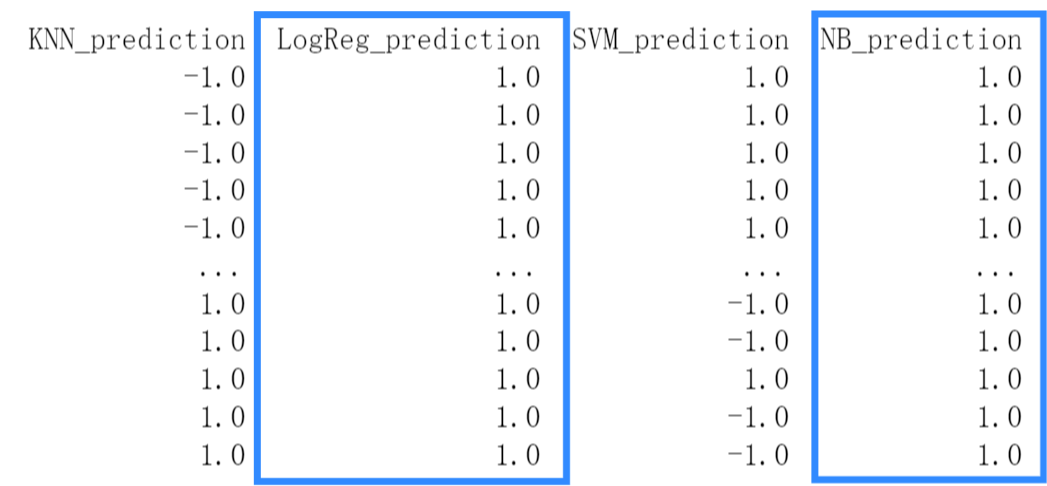
However, during the testing phase, we encountered issues with the logistic regression and Naive Bayes models. Specifically, when dealing with stocks like NVIDIA, which had a significantly higher number of days with price increases than decreases (as shown in the "buy_or_sell" column in the first graph, "1" indicating "increase" and "-1" indicating "decrease"), these models tended to classify all instances as "1" in the "Buy or Sell" results (as shown in the second graph). As a result, the models' predictions lacked meaningful differentiation, despite achieving relatively high accuracy.
Solution: We decided to exclude the logistic regression and Naive Bayes algorithms and incorporate more complex models, namely Decision Tree and Random Forest. These algorithms offer greater flexibility and are better suited to handle the intricacies of the dataset:
from sklearn.model_selection import train_test_split
from sklearn.preprocessing import MinMaxScaler
from sklearn import tree
from sklearn.ensemble import RandomForestClassifier

def Learning(train_df, test_df, factor):
    val_results = collections.defaultdict(int)

    #Set training set and test set
    x=np.array(train_df[['sentiment_score_'+factor]])
    y=np.array(train_df['buy_or_sell'])
    x_train, x_test, y_train, y_test = train_test_split(x, y, test_size = 0.1, random_state = 0)

    #Decision Tree
    dtc = tree.DecisionTreeClassifier(random_state=0)
    dtc.fit(x_train, y_train)
    val_results['Decision Tree'] = dtc.score(x_test, y_test)

    #Random Forest
    forest_reg = RandomForestClassifier(random_state=0)
    forest_reg.fit(x_train, y_train)
val_results['Random Forest'] = forest_reg.score(x_test, y_test) # 0.5

    return val_results