Abstract
After processing the data, sentiment analysis was conducted on the Federal Reserve (the abbreviation of FR will be used throughout the following text) speeches to obtain sentiment scores of the text. Word Cloud analysis was first applied to visualize the sentiment of the FR text. Next, the VADER tool was used to assign scores to each text and observe the relationship between inflation rates. However, the results may be biased due to certain limitations. Alternatively, the Dictionary Method was used to calculate the sentiment scores. We also perform the data merging and correlation matrix analysis for our future data analysis. In the future, we will conduct regression analysis to discuss the relationship between inflation rate and sentiment index scores.
Word Cloud Analysis
Word Cloud represents text data in the form of tags, where the size and colour of each tag reflect the importance of the word. This technique is useful for quickly gaining insight into the most prominent items in a given text by visualizing word frequency as a weighted list. The code below was used to generate world coulds:
import pandas as pd
from wordcloud import WordCloud
import matplotlib.pyplot as plt

# Read the CSV file
df = pd.read_csv('cleaned.csv')

# Create a word cloud from is in the third column
text = ' '.join(df.iloc[:, 2].astype(str))

# Create a WordCloud object
wordcloud = WordCloud(width=800, height=400, background_color='white').generate(text)

# Display the word cloud
plt.figure(figsize=(10, 5))
plt.imshow(wordcloud, interpolation='bilinear')
plt.axis('off')  # Turn off the axis
plt.tight_layout(pad=0)  # Remove padding around the figure
plt.show()
Three speeches from different periods were selected and analysed to identify the different sentiments conveyed by the Federal Reserve. The results displayed various keywords for each period.
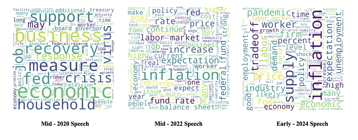
During the pandemic period, concerns were raised about weak consumption and the bankruptcy of many enterprises potentially leading to another global crisis. In a mid-2020 speech titled "Recovery," frequent mentions of words such as "Crisis," "measure," and "support" suggest a preference for stimulus measures to address the economic recession caused by the Covid pandemic.
In mid-2022, inflation surged due to geopolitical uncertainties and supply chain issues stemming from the pandemic. Frequent mentions of words like "Inflation," "Expectation," "fund rate," and "goal" aligned with the Fed's aggressive tight monetary policy aimed at reducing inflation. Although the inflation rate appeared to have returned to normal levels (3.1% in Jan 2024), many lower-income households continued to struggle due to the higher price level.
In an early 2024 speech, high-frequency words such as "inflation," "supply," "unemployment," and "trade-off" indicated that the committee remained cautious about the US inflation rate and adopted a wait-and-see approach.
VADER Analysis
VADER (Valence Aware Dictionary and Sentiment Reasoner) is a sentiment analysis tool that uses a lexicon and rule-based approach to evaluate the sentiment expressed in each text. It is specifically designed to analyse sentiments expressed in social media, but it can also be used to analyse other kinds of texts. VADER works by calculating the percentage of a text that can be categorized as positive, negative, or neutral and produces a compound score that is the sum of the lexicon rating for each word in the text.
Because VADER is easy to implement and does not require training data, it was used to quickly assign sentiment scores to each FR text.
import pandas as pd
import nltk
nltk.download('punkt')
nltk.download('averaged_perceptron_tagger')
nltk.download('maxent_ne_chunker')
nltk.download('words')
nltk.download('vader_lexicon')

#read the file
df=pd.read_csv('cleaned.csv')

#add "ID" column
df.insert(0,"ID",range(1,len(df)+1))

#VADER sentiment analysis
from nltk.sentiment import SentimentIntensityAnalyzer
from tqdm.notebook import tqdm
sia=SentimentIntensityAnalyzer()

#run the polarity score on the entire dataset
res={}
for i,row in tqdm(df.iterrows(),total=len(df)):
    Text=str(row['text'])
    Myid=row['ID']
    res[Myid]=sia.polarity_scores(Text)

#merge the dataframe
vaders=pd.DataFrame(res).T
vaders=vaders.reset_index().rename(columns={'index': 'ID'})
vaders=vaders.merge(df, how='left')
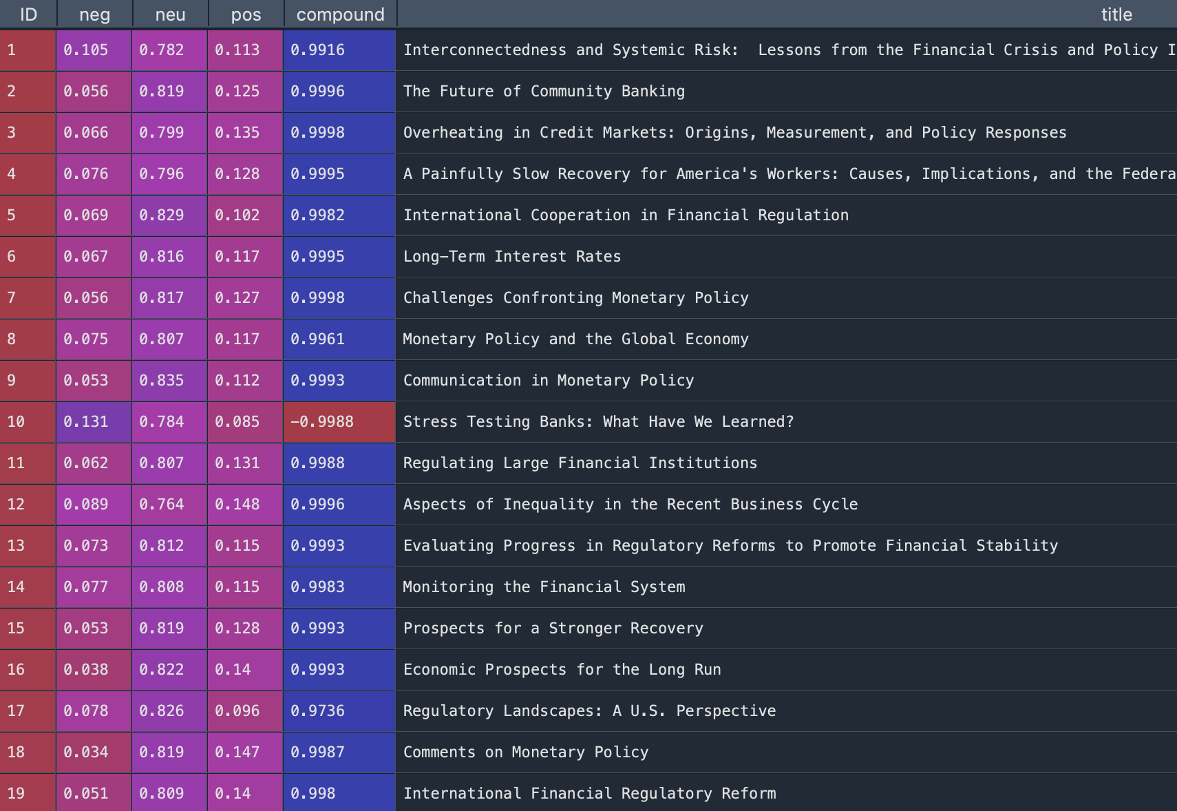
An example of the output is shown below:
We output the results as csv.file. Then, the relationship between VADER scores and inflation rate was visualized through the line chart. From the graph, there is no obviuos realationship between VADER sentiment scores and inflation rate (correlation will be calculated in the later part).
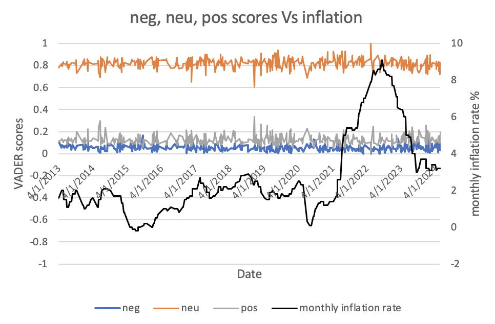
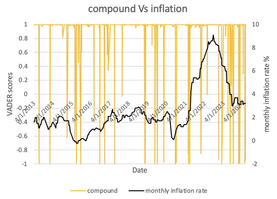
We cannot draw a conclusion because VADER relies heavily on the lexicon, a word may not be accurately classified if it is not present in the lexicon. These limitations may be the possible reasons why VADER did not perform well in FR speeches with complex sentences, which could lead to bias in the results obtained.
Dictionary Method
Alternatively, a Dictionary Method was applied to perform sentiment analysis. Instead of directly importing the built-in dictionary, we created a new customized dictionary that is focused more on economic contents so that the classification and score assignment for FR speech would be more efficient and reliable.
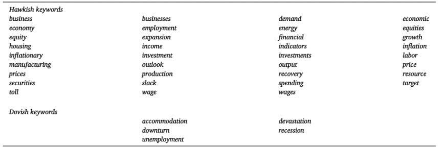
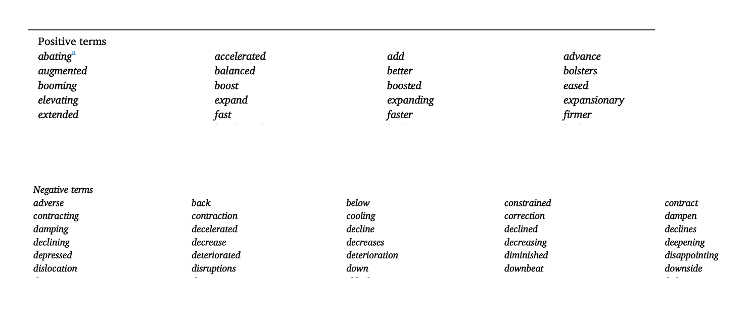
Next, each sentence in the FR speech was classified as positive or negative based on the presence of keywords and polarized terms. Positive terms include the words related to economic boom and proactive action while negative terms encompass the economic recession and hawkish action.
The code is as follows:
# set keyword dic, polarity dic
excel_file = pd.ExcelFile('dictionary_list.xlsx')
dic_list = {}
for sheet_name in excel_file.sheet_names:
    data = pd.read_excel(excel_file,sheet_name)
    dic_list[sheet_name] = data.iloc[:,0].tolist()

keyword_dic = {key: value for key, value in dic_list.items() if key in ['hawkish', 'dovish']}
polarity_dic = {key: value for key, value in dic_list.items() if key in ['positive', 'negative']}

value_list1 = list(keyword_dic.values())
value_list2 = list(polarity_dic.values())


# define a method to screen out the sentences with keyword for each speech through iteration
def get_key_sen(speech):
    sentences = re.split(r'[.?!]\s', speech)
    keyword_sentences = []

    for sentence in sentences:
        words1 = sentence.split()
        for x in words1:
            if x in value_list1[0] or x in value_list1[1]:
                 keyword_sentences.append(sentence)
                 break  # finish internal iteration
        else:
             continue
    return keyword_sentences
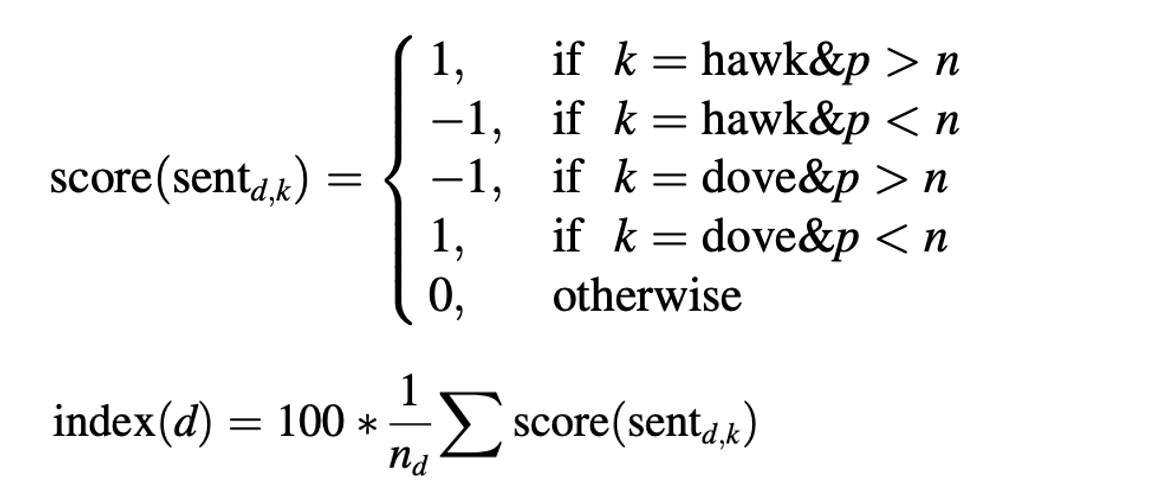
Scores were then assigned to each sentence based on the categorization. If a sentence was categorized as hawkish and had more positive terms than negative terms, a score of +1 was assigned. If it was categorized as hawkish but had more negative terms than positive terms, a score of -1 was assigned. If a sentence was categorized as dovish and had more positive terms than negative terms, a score of -1 was assigned. If it was categorized as dovish but had more negative terms than positive terms, a score of +1 was assigned. Any other case resulted in a score of 0. The sentiment index was calculated by taking the average of the scores for each sentence with the respective keyword dictionary.
The code as follows:
# define a method to categorize each sentence and calculate the amount of polarity words through iteration
def get_sen_scores(keyword_sentences):
    result = []
    for key_sen in keyword_sentences:
        category = ''
        positive_count = 0
        negative_count = 0

        words2 = key_sen.split()  # words2 is a list including strings
        for y in words2:
            if y in value_list1[0]:
                category = 'hawkish'
            elif y in value_list1[1]:
                category = 'dovish'
                break

            index = words2.index(y) # return index of polarity word
            if y in value_list2[0]:
               if index >= 2 and "not" in words2[index-2:index] or index < len(words2)-2 and "not" in words2[index+1:index+3]:
                  positive_count += 1
               else:
                  negative_count += 1
            elif y in value_list2[1]:
               if index >= 2 and "not" in words2[index-2:index] or index < len(words2)-2 and "not" in words2[index+1:index+3]:
                  negative_count += 1
               else:
                  positive_count += 1

        # calculate the sentiment score of each sentence
        sen_score = 0
        if category == 'hawkish':
           if positive_count > negative_count:
              sen_score = 1
           elif positive_count < negative_count:
               sen_score = -1
        elif category == 'dovish':
            if positive_count > negative_count:
                sen_score = -1
            elif positive_count < negative_count:
                sen_score = 1
        else:
            sen_score = 0
        result.append((key_sen, category,positive_count,negative_count,sen_score))
    return result

# define a method to calculate the sentiment score of each speech
def get_speech_scores(result):
    score = [sub_list[4] for sub_list in result]
    sen_num = len(result)
    sentiment_score = round(sum(score)/(sen_num+1) * 100, 2)
    return sentiment_score

# iterate all the speeches
speeches = df['text'].loc[:]
sentiment_index = []

for speech in speeches:
    keyword_sentences = get_key_sen(speech)
    result = get_sen_scores(keyword_sentences)
    sentiment_score = get_speech_scores(result)
    sentiment_index.append(sentiment_score)

#print(sentiment_index)
sentiment_index = pd.Series(sentiment_index) # transfer data into Series type
# standardize the sentiment score
mean_value = sentiment_index.mean()
std_value = sentiment_index.std()
print("mean:", mean_value)
print("sd:", std_value)
standardized_index = (sentiment_index - mean_value) / std_value
print(standardized_index)
df.loc[:,'sentiment_index'] = standardized_index # new column added to df
We output the sentiment index as csv file.
outputpath = 'sentiment_index.csv'
df.to_csv(outputpath,sep=',',index=False,header=True)
The relationship between inflation rate and the sentiment index scores from FR speeches can be observed by visualizing the sentiment index scores.
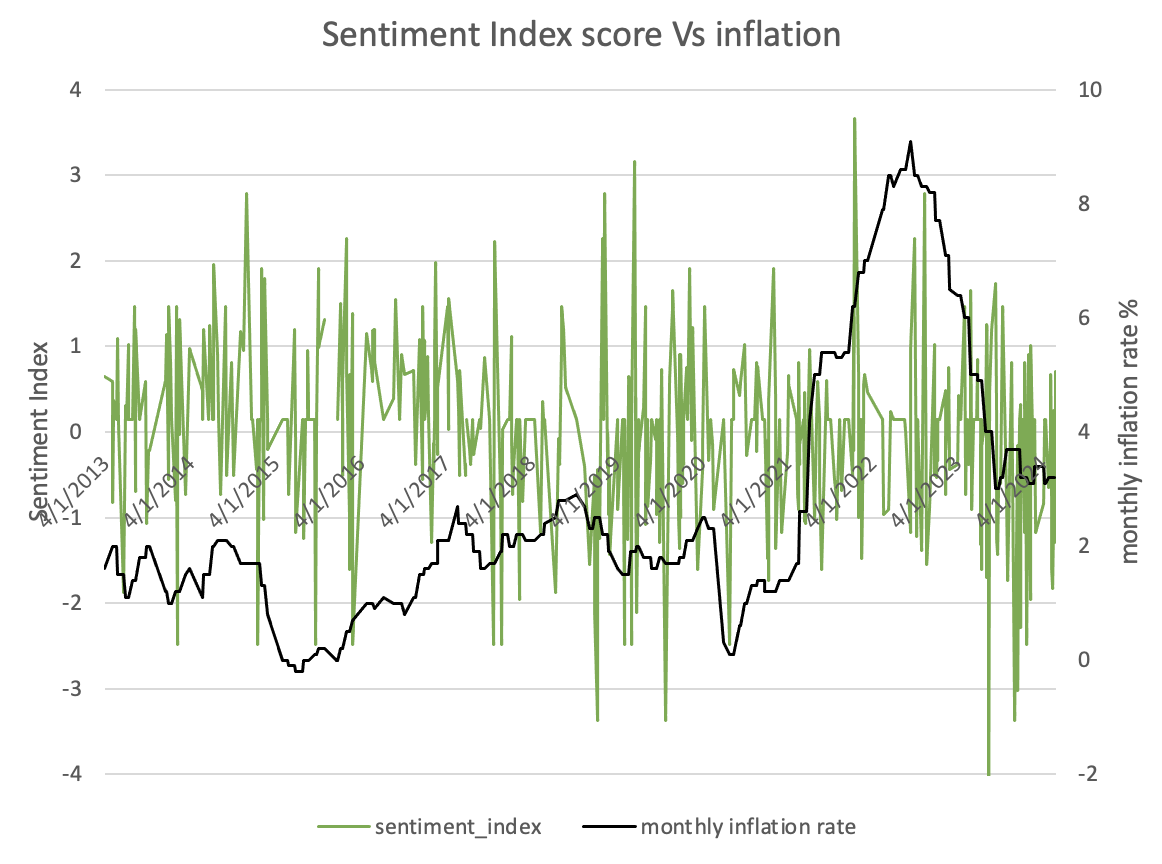
However, though the dictionary method succeeded in calculating the sentiment score, an issue couldn not be ignored is that the efficiency and hashrate of the model is relatively weak since the model utilized lots of iteration, once the data volume is larger the workload for the calculation would also become heavier. Therefore, the optimization of model is one of the future work we should finish.
Data Merging
After we have calculated the VADER scores and Dictionary scores respectively, we merge the scores gotten from the two methods, and then merge it with the inflation rate data. Firstly, we import all datasets that we used:
import pandas as pd
import numpy as np
inflation= pd.read_excel('inflation.xlsx',sheet_name="Sheet3") #import inflation data
score=pd.read_csv('sentiment_index.csv') #import data we got from Dictionary method
vader=pd.read_csv('vaderoutput.csv') #import data we got from VADER method
Before merging the two dataset (gotten from VADER methods and Dictionary methods), we preprocess the data again for merging (eg.convert the ‘date’ variable into date type, only keep the key columns that we want to use, sort the data according to the first key ‘date’ and the second key ‘title’, and create the ‘ID’ column for merging).
score['date']=pd.to_datetime(score['date'])
vader=vader[['title','date','text','neg','neu','pos','compound']]
score = score.sort_values(['date','title'], ascending=[True, True])
score.insert(0, 'ID', range(1, len(score) + 1)) #sort data & insert an "ID" column
vader = vader.sort_values(['date','title'], ascending=[True, True])
vader.insert(0, 'ID', range(1, len(vader) + 1)) #sort data & insert an "ID" column
Then we merge the two sentiment datasets into one on the ‘ID’ columns:
sentiment=pd.merge(score,vader, how='left',on=['ID'])
del sentiment['title_y'],sentiment['date_y'],sentiment['text_y']
sentiment = sentiment.rename(columns={'title_x': 'title', 'date_x': 'date',
                                      'text_x': 'text'})
sentiment['Mdate']=sentiment['date'].dt.to_period('M')
To merge the one sentiment dataset and inflation dataset, we preprocess the data from inflation. And because the predicted variable (inflation rate) is monthly, we also aggregate the sentiment dataset by month to take the mean:
#Preprocess the data from inflation
inflation= inflation[['date','inflation rate']]
inflation['Mdate']=inflation['date'].dt.to_period('M')

#Aggregate the sentiment dataset by month
Msentiment = sentiment[['neg','neu','pos','compound','sentiment_index','date','Mdate']]
Msentiment = Msentiment.groupby(pd.Grouper(key='date', freq='M')).agg({
    'neg': 'mean', 'neu': 'mean','pos': 'mean','compound': 'mean',
    'sentiment_index': 'mean'})
Msentiment = Msentiment.dropna() #drop rows with NaN values
Msentiment['Mdate']=Msentiment.index.to_period('M')
Then we merge the sentiment dataset and inflation dataset on month:
Merge=pd.merge(Msentiment,inflation, how='left',on=['Mdate'])
Correlation matrix
After we merge all datasets, first, we roughly check correlation between the inflation rate and scores gotten from two methods:
#Calculate the correlation matrix without any time lags
Merge_select=Merge[['neg','neu','pos','compound','sentiment_index','inflation rate']]
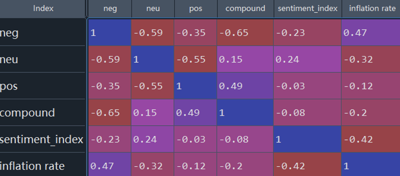
Correlation_matrix = Merge_select.corr().round(2)
From the results, we can see the correlation between the inflation rate and Dictionary method scores (sentiment_index) is -0.42 (which is negative and the degree is moderate). We choose this variables to create lags for furthur analysis.
Since the sentiment score is also likely to reflect future inflation expectations, we create 12 months lags on the sentiment_index:
Merge['sentiment_index1']=Merge['sentiment_index'].shift(+1)
Merge['sentiment_index2']=Merge['sentiment_index'].shift(+2)
Merge['sentiment_index3']=Merge['sentiment_index'].shift(+3)
Merge['sentiment_index4']=Merge['sentiment_index'].shift(+4)
Merge['sentiment_index5']=Merge['sentiment_index'].shift(+5)
Merge['sentiment_index6']=Merge['sentiment_index'].shift(+6)
Merge['sentiment_index7']=Merge['sentiment_index'].shift(+7)
Merge['sentiment_index8']=Merge['sentiment_index'].shift(+8)
Merge['sentiment_index9']=Merge['sentiment_index'].shift(+9)
Merge['sentiment_index10']=Merge['sentiment_index'].shift(+10)
Merge['sentiment_index11']=Merge['sentiment_index'].shift(+11)
Merge['sentiment_index12']=Merge['sentiment_index'].shift(+12)
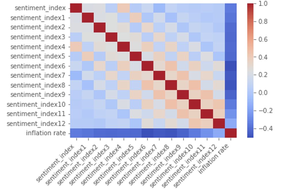
We create the correlation matrix and plot the heat map:
Merge1=Merge.dropna()
Merge_select1=Merge1[[
    'sentiment_index','sentiment_index1','sentiment_index2','sentiment_index3',
    'sentiment_index4','sentiment_index5','sentiment_index6','sentiment_index7',
    'sentiment_index8','sentiment_index9','sentiment_index10','sentiment_index11',
    'sentiment_index12','inflation rate']]
Correlation_matrix1 = Merge_select1.corr().round(2)

#For the heat map
import pandas as pd
import seaborn as sns
import matplotlib.pyplot as plt
#Visualize the matrix of correlation coefficients using seaborn's heatmap function
sns.heatmap(Correlation_matrix1, annot=False, cmap='coolwarm')
plt.xticks(rotation=45, ha='right')
#show the plot
plt.show()
The result is shown below:
Future Discussion
For the next part, we will conduct the regression analysis to further discuss the relationship between inflation rate and sentiment index scores.