Introduction

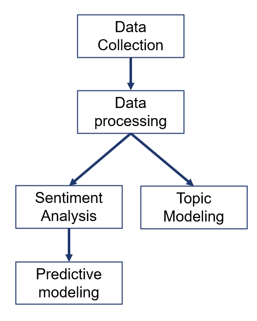
Our project aims to explore the relationship between cryptocurrency market dynamics and construct an effective model for predicting Bitcoin prices by analyzing public opinion information. The following are the concrete steps of our project:

Data Collection

We collected price data from Yahoo Finance and text data from different websites, including Bitcoin Talk, Yahoo Finance and Reddit. The detailed process of crawling has been shown in blog1.

Data Processing

Bitcoin Price

Instead of using the bitcoin price directly, we used the rise and fall of the price as a dummy variable. It is more practical to predict the price trend than to predict the specific price directly. Price trends are more actionable for traders as they can be used to develop buy or sell strategies.

Price change = 1 while price rises

Price change = 0 while price falls

Sentiment Score

For the sentences we crawled from the websites, we gave each a sentiment score using TextBlob() and and averaged the scores for each day. The code is as follows:

df['title'] = df['title'].astype(str)
df['polarity'] = df['title'].apply(lambda x: TextBlob(x).sentiment.polarity)
df['subjectivity'] = df['title'].apply(lambda x: TextBlob(x).sentiment.subjectivity)

Topic Modeling

We wanted to confirm if the core topic of the data is closely related to the Bitcoin price we want to predict, but the amount of data is too large to analysis. So we used the Topic Modeling method. The code of Topic Modeling is as follows:

# cv
cv = CountVectorizer(stop_words = 'english', min_df = 0.01, ngram_range = (1,2))
corpus_cv = cv.fit_transform(data['title'])
corpus_cv.toarray()
feats = cv.get_feature_names_out()
corpus_array = corpus_cv.toarray()
df = pd.DataFrame(corpus_array, columns = feats, index = sources)

# tfidf
tfidf = TfidfVectorizer(stop_words = 'english', min_df = 0.01, ngram_range = (1,2))
corpus_tfidf = tfidf.fit_transform(data['title'])
feats_tfidf = tfidf.get_feature_names_out()
corpus_array_tfidf = corpus_tfidf.toarray()
df_tfidf = pd.DataFrame(corpus_array_tfidf, columns = feats_tfidf, index = sources)

lda1 = LatentDirichletAllocation(n_components = 5, max_iter = 10, learning_method = 'online', learning_offset = 50., n_jobs=6,random_state = 2)
lda1.fit(corpus_cv)
lda2 = LatentDirichletAllocation(n_components = 5, max_iter = 10, learning_method = 'online', learning_offset = 50.,n_jobs=6, random_state = 2)
lda2.fit(corpus_tfidf)

By using LDA model, we clustered news articles into different groups with specific topics. The following two graphs present the topics generated by LDA with TF-IDF and Bow. Obviously, the TFIDF version is better at finding the core topics. Then we concluded that TFIDF is the appropriate word vector model that fits well in the LDA model.

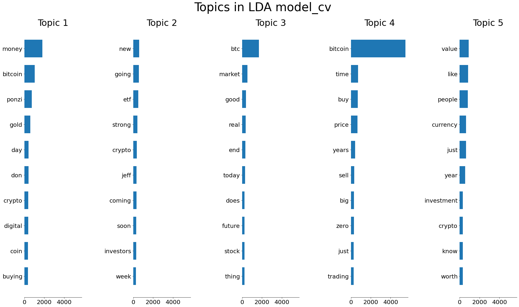
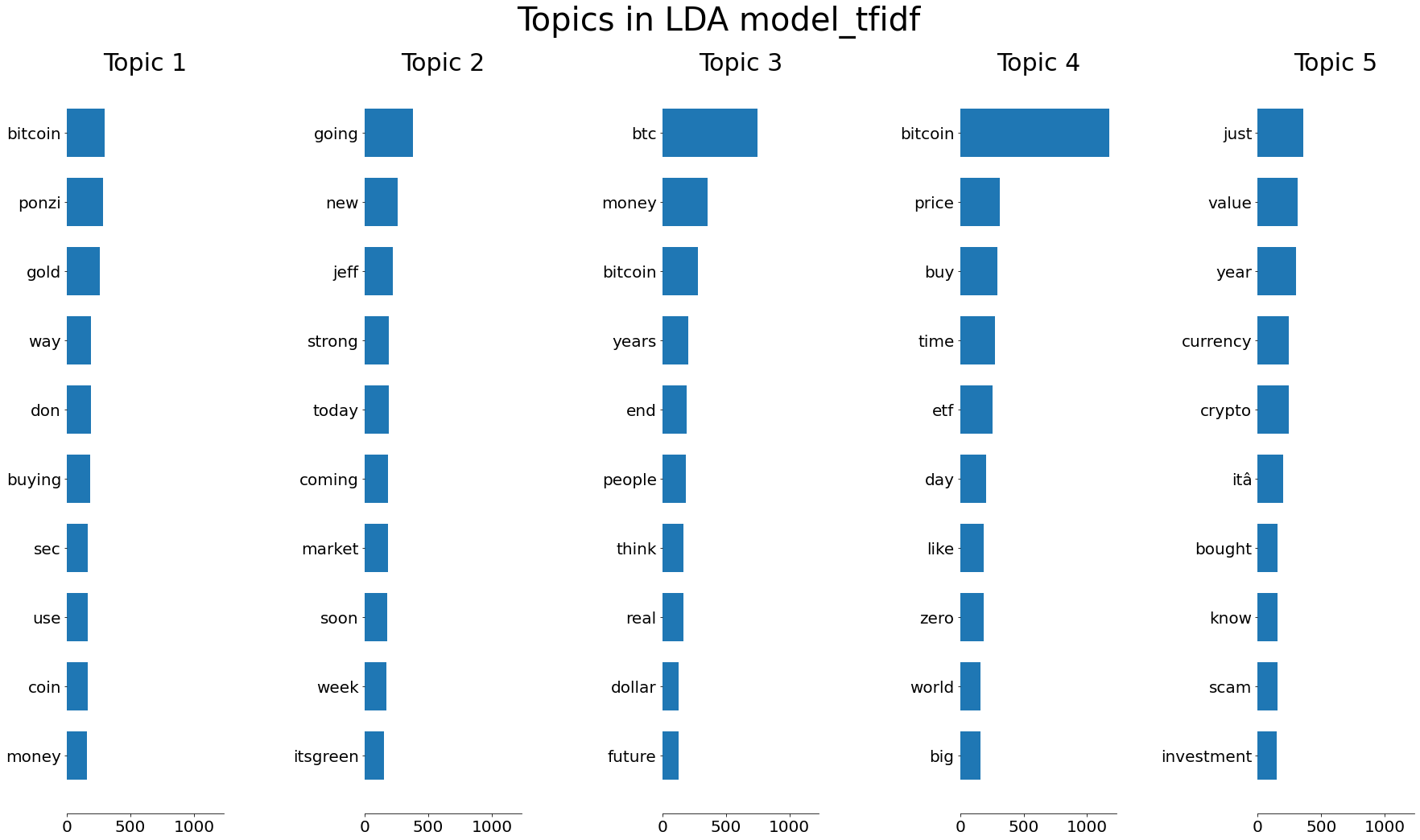
The consistency within groups would make it easier for us to interpret the meaning of features such as sentiment scores of the news articles. The topics are all related to bicoins which are exactly what we are looking for in this project.

Predictive Modeling

In our improved logistic model, we used grouped sentiment score, normalized trading volume and the UBL factor(which will be introduced in blog3) as independent variables and the price change as the dependent variables. The code we used is as follows:

# Logistics regression
X = df_final1[['polarity_scale_Positive','polarity_scale_Strongly Negative', 
               'polarity_scale_Strongly Positive', 'volume_scaled', 'UBL']]  
y = df_final1['price_change'] 

X_train, X_test, y_train, y_test = train_test_split(X, y, test_size=0.2, random_state=42)
model = LogisticRegression()
model.fit(X_train, y_train)

# Predict on test data
y_pred_proba = model.predict_proba(X_test)[:, 1]

# Calculate ROC-AUC score
roc_auc = roc_auc_score(y_test, y_pred_proba)
print("ROC-AUC Score:", roc_auc)

The ROC curve is showing as follow:

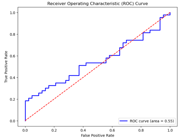
As the AUC score is 0.54, which is bigger than 0.5, our model is effective in predicting the bitcoin price.