By Group "N.5". We are N.5, aiming to discover investment opportunities hiding behind market factors.
General thought of Project
The issue of stock market prediction has always attracted great interest from both academic and business communities. But are financial markets really predictable? Traditional finance is based on the random walk and efficient market hypothesis. And according to the efficient market hypothesis theory, stock prices movement depend on emerging of information (such as news) rather than on past or future stock prices.
Many studies have also shown that financial markets are not a completely random process. To some extent, there is a degree of predictability in financial markets. For example, it is true that we cannot predict the emergence of new information in the market, but it is possible to capture some signs from social networking media (Twitter, Facebook, other blogs, etc.) and use them to predict, to some extent, future changes in sentiment and information in the economy and society.
In a paper Twitter mood predicts the stock market, researchers at Indiana University and Manchester University used tweets posted by users on Twitter to analyze sentiment through two sentiment analysis models, namely OpinionFinder and Google-Profile of Mood States (GPOMS), to capture and analyze changes in public sentiment.
Different from predicting the movement of individual stocks, we are planning to focus on forecasting the movement of Nasdaq 100 stock index. By analyzing the sentiments of all stocks in a specific time period, we will forecast the overall Nasdaq 100 stock index up or down movement. Then, we will figure out the best model for accuracy prediction.
Data Resource and Data Scraping
-
Tweets Data with Nasdaq100 tickers cashtag
-
Historical financial Nasdaq100 data from Yahoo! Finance
![]()
Nasdaq100 Data
We get the Nasdaq100 ticker weights online, see the example below:
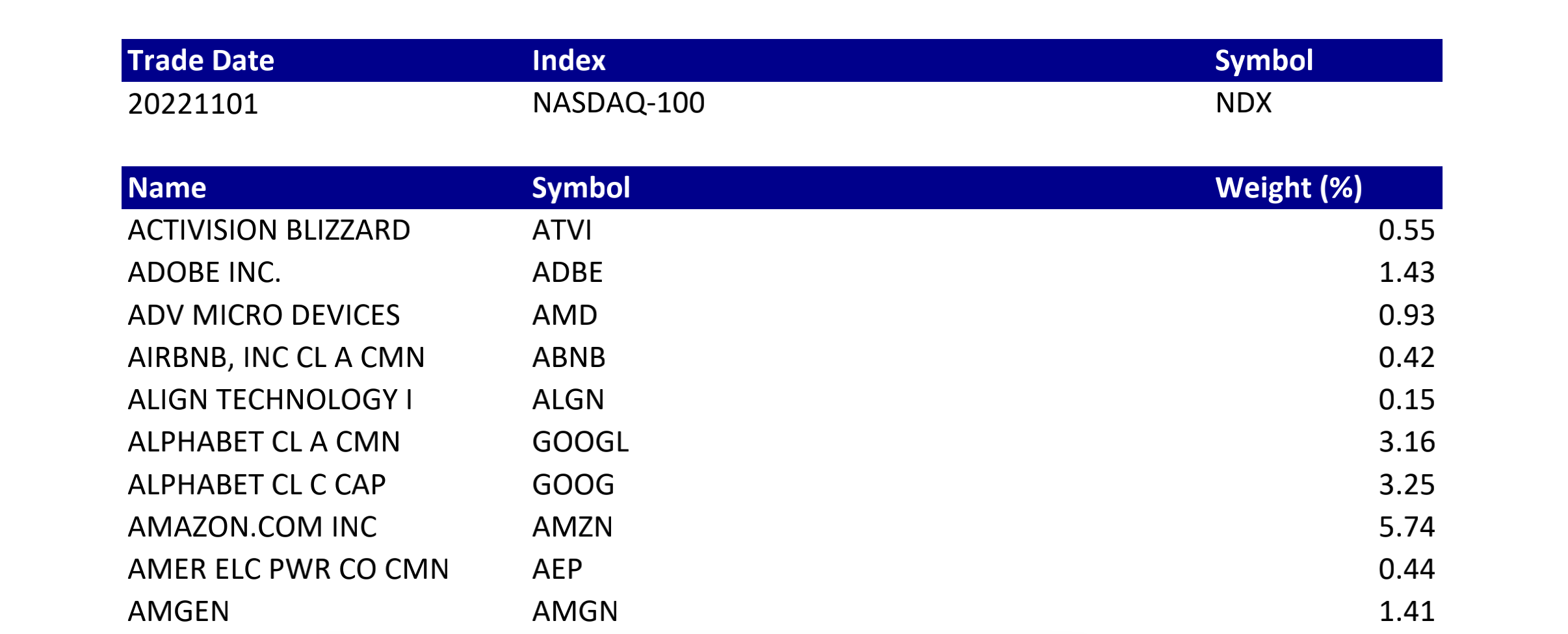
Then we import pdfplumber to Plumb this PDF file for detailed information about each text character, rectangle, and line. After some data cleaning, we transfer the pdf into csv version.
Tweets Data
In this step, we want to get tweets that contained Nasdaq 100 ticker cashtag and cleaned the data for further use. In order to get enough data for our research, we decide to scrape a half year tweets and financial data from 2022-07-01 to 2022-12-31. However, we tried different ways to get the tweets data.
At first, we tried followthehashtag.com, a Twitter search analytics and business intelligence tool. We expect to get the negative and positive tweets with cashtags as following. However, the information on the website is outdated, and difficult to sign in.
Then, we tried to use Twitter API, which is the official tweets scraping tool. However, Tweepy does not allow recovery of tweets beyond a week window, so historical data retrieval is not permitted, so it is hard for us to retrieval the specific time period we want. Also, there are limits to how many tweets you can retrieve from a user's account.
After failure in using twitter API, we tried tweet scraper, but is incompatible with current software, and there will have too many missing data, and incorrespond data after web scraping.
Finally, we choose snscrape, a scraper for social networking services. It scrapes things like user profiles, hashtags, or searches and returns the discovered items. The code we use is as follows:
#Extracting the tweets by snscrape
df_lst = []
for stock in tqdm(cashtags):
    i = stock
    query = f'(from:{i}) until:2022-12-31 since:2022-07-01'
    tweets = []
    limit = 50000
    for tweet in sntwitter.TwitterSearchScraper(query).get_items():
        # print(vars(tweet))
        # break
        if len(tweets) == limit:
            break
        if tweet.lang != 'en':
            continue
        else:
            tweets.append([stock, tweet.date, tweet.username, tweet.user.followersCount, tweet.content,tweet.likeCount,tweet.lang])
    df_stock = pd.DataFrame(tweets, columns=['cashtag','Date', 'User', 'Number of Followers', 'Tweet','likes','languages'])
    df_lst.append(df_stock)
df=pd.concat(df_lst)

df.to_parquet(file_path+'/old_tweets.pq')
df.to_csv(file_path+'/old_tweets.csv')
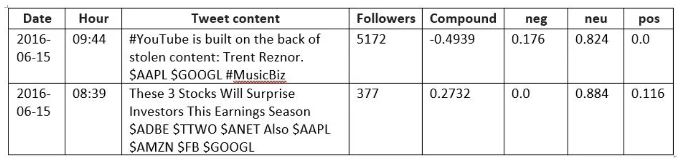
Then we get the half year tweets data, that include name of the hashtag, date, Tweets, etc.

Stock Data
We got the Nasdaq 100 stock price data from Yahoo! Finance.
stock_pr = []
for stock in tqdm(ndx_100['ticker']):
    data_df = yf.download(stock, start="2022-07-01", end="2022-12-31")
    data_df['cashtag'] = '$'+stock
    # get stock info
    stock_pr.append(data_df)

stock_pr_df = pd.concat(stock_pr)
stock_pr_df.to_csv(file_path+'/stock_price.csv')
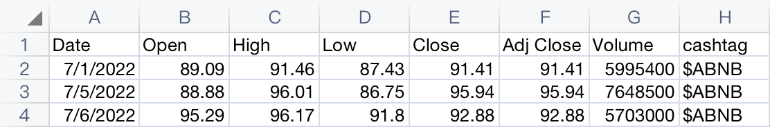
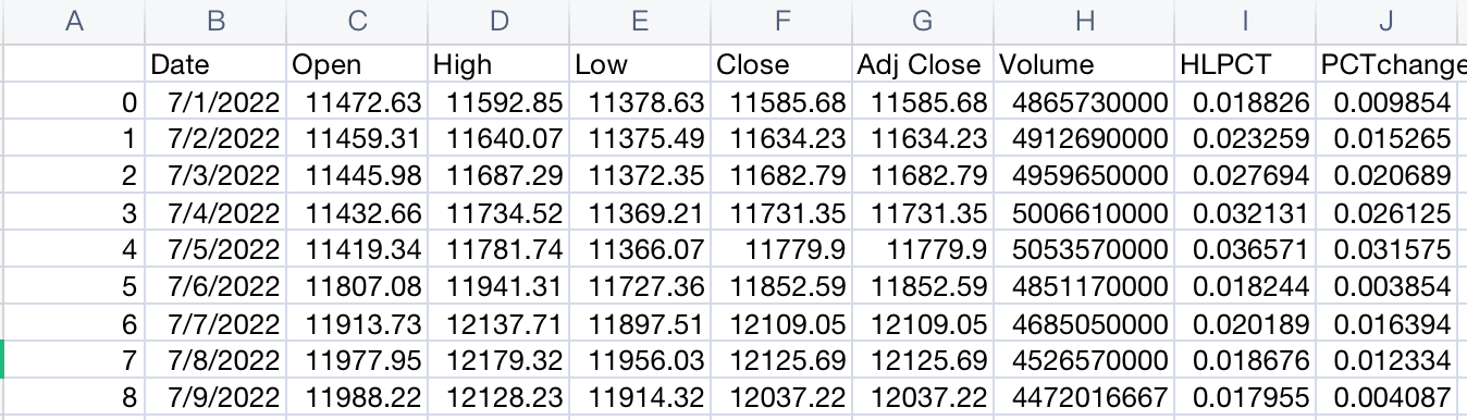
The following example is the CSV file we download from Yahoo! Finance, it contains basic information including the open and close daily price of Nasdaq 100 tickers.
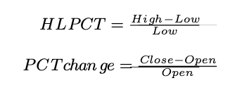
Then we create two new roles, "HLPCT" and "PCTchange". The formula and codes in the following:
ndx = yf.download('^NDX', start="2022-07-01", end="2022-12-31")
ndx.reset_index(inplace = True)

helper =pd.DataFrame({'Date':pd.date_range(start=ndx['Date'].min(),\
end=ndx['Date'].max(),freq='1d')})

ndx = pd.merge(helper,ndx,on = 'Date',how = 'left')

ndx[ndx.columns.to_list()[1:]]=ndx[ndx.columns.to_list()[1:]].apply(lambda x:\
x.interpolate(),axis=0)

ndx['HLPCT'] = (ndx['High']-ndx['Low'])/ndx['Low']
ndx['PCTchange'] = (ndx['Close']-ndx['Open'])/ndx['Open']
ndx.to_csv(file_path+'/nasdaq100.csv')
Result we obtain:
Data Cleaning and Sentiment Analysis
In this part we will guide you through our exploration of twitter text analysis.
Text Processing
First, we decide to transform all texts corresponding to all stocks for each day into sentiment scores, then manually multiplied and transformed into 1-dimensional features to predict Nasdaq 100 Index up or down pricing.
However, after training the machine learning classifiers with the data (Including logistic Regression, Support Vector Machine, Decision Tree, and Random Forest etc), the results, after running each of the stocks through each of the 5 binary classifiers and cross-validation, accuracy of each classifier was just between 45% to 55%. We did not recognize any connection between sentiment score on twitter and Nasdaq 100 Index ups and downs.
Fix the problem: We found that since NASDAQ 100 index is a weighting of 100 stocks, there will be some steps missing when learning the total ups and downs directly from the characteristics of 100 stocks. It is to use 1 model to predict the up and down values of 100 stocks, and then weight and sum the predicted values to get the final NASDAQ up and down, instead of directly predicting the overall NASDAQ up and down (because the weights and summation formula are known). Also, with only one model, there will be more training data.
Choosing Sentiment Analysis
Since the number of tweets and the length of text are not fixed, we want to use word frequency statistics such as tf-idf are used to transform the features into fixed-length ones, or use rnn deep learning models for processing indefinite length sequences.
We simplified the problem to a binary classification. When we get the prediction of the index price for next day, if it shows positive, then we assign it as up movement with 1, if it is negative, we assign it -1 as downward movement. As a result, the performance of the models were much better.
Later, we found that Vader is good for sentiment analysis of social media text data, so we started to learn the principle and usage of this package, and finally used it for sentiment analysis. Below is code of the data processing stage using Vader:
Tweet = tweets.drop(columns=['Unnamed: 0']).copy()
Tweet = Tweet.loc[Tweet['Tweet'].isna() == False]

Tweet['Tweet'] = [re.sub(r'http\S+','',i) for i in Tweet['Tweet']]
Tweet['Tweet'] = [re.sub(r"[$]\S+", " ", i) for i in Tweet['Tweet']]

#The function for assigning the sentiment score for each tweet
def sentimentScore(Tweet):
    analyzer = SentimentIntensityAnalyzer()
    results = []
    for sentence in Tweet:
        vs = analyzer.polarity_scores(sentence)
        results.append(vs)
    return results

df_results = pd.DataFrame(sentimentScore(Tweet['Tweet']))

Tweet.reset_index(inplace = True, drop = True)
Tweet = pd.concat([Tweet,df_results],axis = 1)
#Tweet.drop(columns=['Unnamed: 0'],inplace=True)
Tweet.to_csv(file_path_2+'/tweets_with_senti_scores.csv',index=False)
Tweet = Tweet.loc[Tweet['compound'] != 0]
Tweet['Date'] = pd.to_datetime(Tweet['Date']).apply(lambda x:\
x.strftime('%Y/%m/%d'))
Tweet['Date'] = pd.to_datetime(Tweet['Date'])
Tweet['log_followers'] = np.log(Tweet['Number of Followers'])
Tweet = Tweet.loc[Tweet['Number of Followers'] != 0]
Tweet['Compound_multiplied'] = Tweet['log_followers']*Tweet['compound']

senti_score=Tweet[['cashtag','Date','compound','Compound_multiplied']].groupby \
(by=['cashtag','Date']).mean()
senti_score = senti_score.reset_index()
Combine the data together:
stock_full = senti_score.merge(stock_pr_df,on=['cashtag','Date'],how='outer')
stock_full = stock_full.loc[stock_full['compound'].isna() == False]
stock_price_info = ['Open','High','Low','Close','Adj Close','Volume']
stock_full[stock_price_info] = stock_full[stock_price_info].apply(lambda x: \
x.interpolate(),axis=0)
stock_full['HLPCT'] = (stock_full['High']-stock_full['Low'])/stock_full['Low']
stock_full['PCTchange'] = (stock_full['Close']-stock_full['Open'])\
/stock_full['Open']

stock_full = stock_full.merge(ndx_100,left_on='cashtag',right_on='Cashtags')
stock_full.drop(columns =['Cashtags'],inplace = True)

stock_full[['PCTchange_lag_1']] = stock_full.groupby(by=['cashtag'])\
[['PCTchange']].shift(-1)

stock_full.dropna(subset=['PCTchange_lag_1'],inplace = True)
stock_full.to_csv(file_path_2+'/stock_full.csv',index=False)
Modeling
In this part, we will simply interpret the model we pick and the performance of the models. More results of the modeling and future improvements can be seen in the report.
We first define the data_train and data_test:
data=stock_full[['Date','ticker','compound','Compound_multiplied','Close','HLPCT',
'Volume','PCTchange','Weights','PCTchange_lag_1']]
data_train = [data.loc[v[:round(len(v)*0.8)]] for g, v in data.groupby('ticker')\
.groups.items()]
data_train = pd.concat(data_train)
data_test = [data.loc[v[round(len(v)*0.8):]] for g, v in data.groupby('ticker')\
.groups.items()]
data_test = pd.concat(data_test)
The Lecture notes also mentions Neural Networks, ISTM, BERT, and other models, but they are more complicated to use, thus we first tried traditional machine learning model. Replace the classification model with regression model where the prediction target is a specific up or down value instead of plus or minus 1 (the prediction target will be more continuous), then convert the model prediction results (real numbers) to +1 or -1 (Nasdaq 100 Index ups or downs) and then calculate the accuracy.
Different from the model we expect to use during the planning stage, We use models including Linear regression, Decision Tree, SVM, XGboost, and lightGBM. Before we write the code, we also install the sklearn package on python, and import those package at the beginning of code writing:
from sklearn.tree import DecisionTreeRegressor
from sklearn.linear_model import LogisticRegression
from sklearn.svm import SVR
from sklearn import linear_model
from lightgbm import LGBMRegressor
from xgboost import XGBRegressor
The code of the five model can be seen below:
#Linear Regression
def LR(y_train,x_train,x_test,y_test):
    clf = linear_model.LinearRegression()
    clf.fit(x_train,y_train)
    #print(clf.score(x_test,y_test))
    return clf.predict(x_test)

#Decision Tree regressor
def DTreg(y_train,x_train,x_test,y_test):
    clf = DecisionTreeRegressor()
    clf = clf.fit(x_train,y_train)
    #print(clf.score(x_test,y_test))
    return clf.predict(x_test)

#SVR
def SVRreg(y_train,x_train,x_test,y_test):
    clf = SVR()
    clf = clf.fit(x_train,y_train)
    #print(clf.score(x_test,y_test))
    return clf.predict(x_test)

#XGboost
def XGBreg(y_train,x_train,x_test,y_test):
    clf = XGBRegressor(random_state=123)
    clf = clf.fit(x_train, y_train)
    #print(lgb.score(x_test,y_test))
    return clf.predict(x_test)

#LightGBM
def lgb(y_train,x_train,x_test,y_test):
    lgb = LGBMRegressor(random_state=123)
    lgb = lgb.fit(x_train, y_train)
    #print(lgb.score(x_test,y_test))
    return lgb.predict(x_test)
Then we split the stock_full data as train and test sets in order to evaluate the performance of machine learning algorithm.
x_train = np.array(data_train[['compound','Compound_multiplied','HLPCT',\
'Volume','PCTchange']])
y_train = np.array(data_train['PCTchange_lag_1'])

x_test = np.array(data_test[['compound','Compound_multiplied','HLPCT',\
'Volume','PCTchange']])
y_test = np.array(data_test['PCTchange_lag_1'])
To get the performance of each model
We create confusion matrix for further results analysis. Below is an example of the linear regression model, By changing the first line LR to different model definitions, we will get different results for each model, and compare the accuracy between different model.
y_pred = LR(y_train,x_train,x_test,y_test)
y_pred_operations = y_pred.copy()
data_test['pred_PCTchange'] = y_pred_operations
data_test['NDX_pred_PCTchange'] = data_test['pred_PCTchange']*data_test['Weights']

y_pred_NDX = data_test.groupby(by='Date').sum()['NDX_pred_PCTchange']
y_pred_NDX = y_pred_NDX.reset_index()

ndx['Date'] = pd.to_datetime(ndx['Date'])

#y_NDX = ndx.loc[ndx['Date'].isin(y_pred_NDX['Date']),['Date','PCTchange']]
y_NDX = ndx.loc[ndx['Date'].isin(y_pred_NDX['Date']),['Date','PCTchange']]

y_pred_NDX['NDX_pred_PCTchange'][y_pred_NDX['NDX_pred_PCTchange'] >= 0] = 1
y_pred_NDX['NDX_pred_PCTchange'][y_pred_NDX['NDX_pred_PCTchange'] < 0] = -1
y_test_NDX = y_NDX.copy()
y_test_NDX['PCTchange'][y_test_NDX['PCTchange'] >= 0] = 1
y_test_NDX['PCTchange'][y_test_NDX['PCTchange'] < 0] = -1
score = accuracy_score(y_test_NDX['PCTchange'], y_pred_NDX['NDX_pred_PCTchange'])

confusion_matrix = metrics.confusion_matrix(y_test_NDX['PCTchange'], y_pred_NDX['NDX_pred_PCTchange'])
cm_display = metrics.ConfusionMatrixDisplay(confusion_matrix = confusion_matrix, display_labels = [False, True])
cm_display.plot()

targetnames = ['Down','Up']
print(classification_report(y_test_NDX['PCTchange'], y_pred_NDX['NDX_pred_PCTchange'],target_names = targetnames))

RocCurveDisplay.from_predictions(y_test_NDX['PCTchange'], y_pred_NDX['NDX_pred_PCTchange'])
print(score)
Below is an example of the confusion matrix and classification report we get for the linear regression model, we can see the overall accuracy of model.
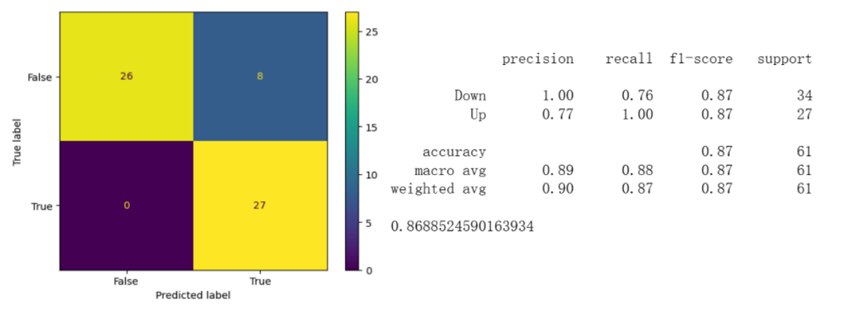
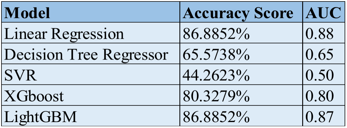
After running all of the models, we combine all of the model together and it shows the clear result of each model's accuracy.