Data processing and Linear Regression in Python (by Group "NLP Intelligence")

By Group "NLP Intelligence"

We have collected text data and transformed text into numbers through the process posted in the previous blogs. To investigate the correlation between investors’ sentiment and price return, we try to merge text and financial data frames, run the regression model, and print the regression results. Hence, in this blog, we would like to show you the details about data merging, data cleaning, and regression processing.

Data merging

Before we merge the data frames, we have to get the daily average sentiment index. The reason is that there may be more than one post each day, and we have collected separate sentiment indexes for each post.

We used the following code to get the daily average sentiment index and remove the duplicates:

#get daily average SentimentScores
New_SentimentScores = SentimentScores[['Date','compound']]
New_SentimentScores['avg_compound'] = New_SentimentScores['compound'].groupby(New_SentimentScores['Date']).transform ('mean')
del New_SentimentScores['compound']

New_SentimentScores = New_SentimentScores.drop_duplicates()
New_SentimentScores.head()

After getting the daily average sentiment index, we could merge the text and financial data frames based on the column “date”.

Regression_Data = pd.merge(StockReturn, New_SentimentScores, how='left', on=['date'])
# pd: import pandas as pd
# how: put dataframe StockReturn on the left
# on: based on the same date

Data winsorization, standardization, normalization

Because we have data from deep learning, we try to standardize these data to improve their quality. There are a few outliers in the data, so we winsorized data before the standardization. If we do not conduct the winsorization, the outlier will affect the standardization, and we may not get a satisfactory result from standardization.

# Winsorize
SentimentScores['wins_compound'] = \
    SentimentScores['compound'].\
    clip(
        upper=SentimentScores['compound'].quantile(0.99),\
        lower=SentimentScores['compound'].quantile(0.01))

# Standardize
SentimentScores['std_compound'] = preprocessing.scale(SentimentScores['wins_compound'])

# check the mean and std after processing
np.mean(SentimentScores['std_compound'], axis=0)
np.std(SentimentScores['std_compound'], axis=0)

Then, we can take a look at the processed result by the following codes:

SentimentScores['std_compound'].quantile([0, 0.01, 0.25, 0.5, 0.75, 0.99, 1])
SentimentScores['std_compound'].hist()

Because we want to try our best to unify the work of each part so as to cooperate with group members better. After the standardization, we re-normalized the data to an interval from -1 to 1 by the following codes:

SentimentScores['nor_compound'] = \
    (SentimentScores['std_compound'] - \
     SentimentScores['std_compound'].min()) / \
    (SentimentScores['std_compound'].max() - \
     SentimentScores['std_compound'].min()) * 2 - 1
SentimentScores['nor_compound']

Data cleaning: remove null values

When acquiring data, some data may not be available, or the data itself may not exist, resulting in null values. If we don't remove the null values, we will get the error below.

Picture1 showing

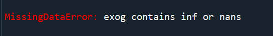
We can use the following code to remove null values:

print(Regression.isnull()) 
Regression.dropna(how='any', axis=0, inplace=True)

Generate new variables

Based on our regression models, we would like to generate two variables first. The first one is a dummy variable called “After_DiDi”. It represents whether the date of each data is after DiDi’s delisting or not. If it’s after DiDi’s case, it will be one; otherwise, it will be zero.

We try to use this variable to explore the potential effect of DiDi’s delisting on the other U.S.-listed China Concept Stocks and to fit the market condition better.

#add a dummy variable
threshold = '2021-07-02'
After_DiDi = np.where(Regression_Data.date >= threshold, 1, 0)
Regression_Data['After_DiDi'] = After_DiDi
del threshold, After_DiDi

Another variable we generated is “sentiment_tag” which is a categorical variable. We would like to transform the sentiment index (continuous floating numbers from -1 to 1) to a categorical variable (from 'Strongly negative' to 'Strongly positive') and encode the labels (from 1 to 5).

We have tried the regression model with sentiment index and got a significant result. But we convert the variable to improve our regression model because the coefficient of a categorical variable with label encoding is much more interpretive for readers.

# change the continuous floating number to a categorical variable
def judge_type(x):
    if x < -0.6:
        a='Strongly negative'
    elif -0.6 <= x < -0.2:
        a='Negative'
    elif -0.2 <= x < 0.2:
        a='Neutral'
    elif 0.2 <= x < 0.6:
        a='Positive'
    elif 0.6 <= x :
        a='Strongly positive'
    else:
        a=''
    return a
Regression_Data['sentiment_label'] = Regression_Data['avg_compound'].apply(lambda x: judge_type(x))

# Label Encoding
def judge_tag(x):
    if x < -0.6:
        a=1
    elif -0.6 <= x < -0.2:
        a=2
    elif -0.2 <= x < 0.2:
        a=3
    elif 0.2 <= x < 0.6:
        a=4
    elif 0.6 <= x :
        a=5
    else:
        a=''
    return a
Regression_Data['sentiment_tag'] = Regression_Data['avg_compound'].apply(lambda x: judge_tag(x))

In addition, our model includes some interaction terms. Adding interaction terms can be implemented very simply with the following code:

# Add interaction terms
Regression['sentiment_tag_After_DiDi'] = Regression['sentiment_tag']*Regression['After_DiDi'] 
Regression['S&P 500_After_DiDi'] = Regression['S&P 500']*Regression['After_DiDi']

Finally, we got the data that could be put into the regression model.

How to implement linear regression in Python

Usually, we choose STATA, R, or SPSS to implement linear regression. But in this project, we tried how to implement linear regression in Python.

import statsmodels.api as sm
Regression_1 = Regression[['Price Return', 'sentiment_tag’, 'S&P 500']] # regression dataset

# dependent variable
y = Regression_1.iloc[:, 0].reset_index(drop=True) 

# explanatory and control variables
x = Regression_1.iloc[:, 1:3].reset_index(drop=True)
x = sm.add_constant(x) # Add intercept term

# linear regression
model_1_1 = sm.OLS(y, x).fit()

# print
print(model_1_1.summary())

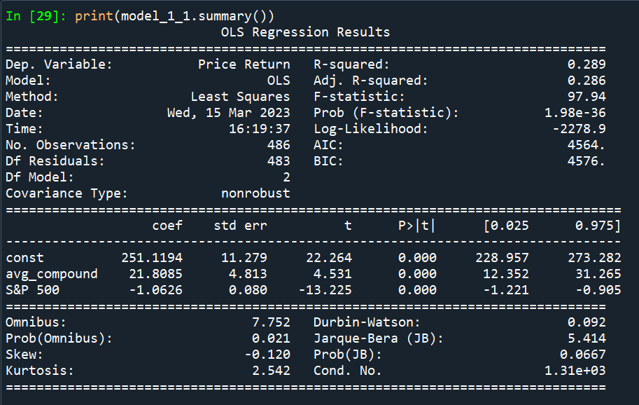
Presentation of regression results

The result printed by Python is the following figure. It can only print each regression result separately. And there is no asterisk shown, so we can only use the t-value and p-value to identify the significance.

Picture2 showing

Therefore, we find another method to combine our regression results on the same page and show the asterisks to present the significance more intuitively. One of our new presentations of regression results is the following figure.

Picture3 showing

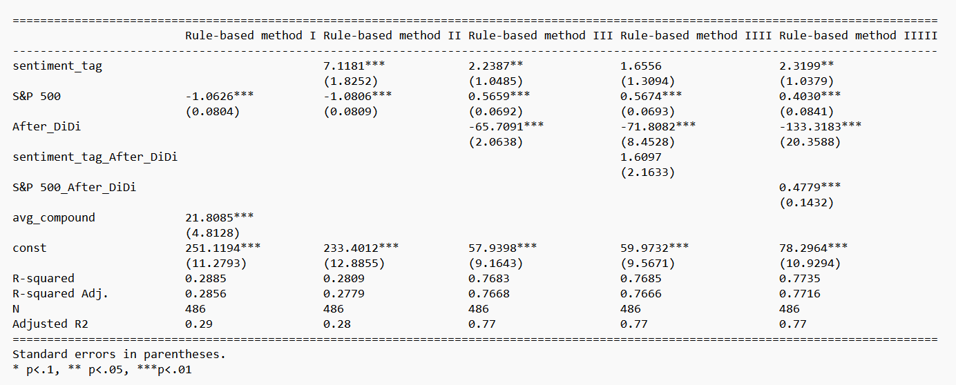
We can use the following code to implement the presentation:

from statsmodels.iolib.summary2 import *

# only Rule-based method
whole_result = \
    summary_col(
        [model_1_1, model_1_2, model_1_3, model_1_4, model_1_5],
        stars=True,
        float_format='%0.4f',
        model_names=['Rule-based method', 'Rule-based method', 'Rule-based method', 'Rule-based method', 'Rule-based method'],
        info_dict={'N': lambda x: "{0:d}".format(int(x.nobs)), 'Adjusted R2': lambda x: "{:.2f}".format(x.rsquared_adj)},
        regressor_order=['Intercept', 'sentiment_tag', 'S&P 500', 'After_DiDi', 'sentiment_tag_After_DiDi', 'S&P 500_After_DiDi'])
whole_result

# only Deep Learning method
whole_result = \
    summary_col(
        [model_2_1, model_2_2, model_2_3, model_2_4, model_2_5],
        stars=True,
        float_format='%0.4f',
        model_names=['Deep Learning Method', 'Deep Learning Method', 'Deep Learning Method', 'Deep Learning Method', 'Deep Learning Method'],
        info_dict={'N': lambda x: "{0:d}".format(int(x.nobs)), 'Adjusted R2': lambda x: "{:.2f}".format(x.rsquared_adj)},
        regressor_order=['Intercept', 'sentiment_tag', 'S&P 500', 'After_DiDi', 'sentiment_tag_After_DiDi', 'S&P 500_After_DiDi'])
whole_result