By Group "Processors"
Objective
In this blog, we will explore the relationship between the sentiment of social discussion and bitcoin price. We mainly use the social media comments as the data source since they normally tend to be more emotional and subjective. Thus, they make a better source for sentimental analysis.
We will walk through the entire process using the data scraped from Conversation under BTC-USD at Yahoo Finance as an example.
Date preprocess
First thing we do after we read both price data and text data into Pandas dataframe separately is to change both date format into '%Y-%m-%d' format based on the datetime.now function in datetime.datetime.
for i in range(0,len(p_df['Date'])):
    p_df['Date'][i] = (datetime.now() - timedelta(i+1)).strftime('%Y-%m-%d')

for i in range(0,len(d_df['date'])):
    days_age = int(d_df['date'][i][:2])
    d_df['date'][i] = (datetime.now() - timedelta(days_age)).strftime('%Y-%m-%d')
We will first deal with the text data. The TextBlob library is used to calculate the sentiments score for each comment. The .polarity method will return a score of how positive the text is within the range from -1 to 1, with 1 being the most positive.
We will then split the score into one of the five classification as follow:
- Strongly Positive: [0.5, 1]
- Positive: (0, 0.5)
- Neutral: [0, 0]
- Negative: [-0.5, 0)
- Strongly Negative: [-1, -0.5)
cmt_to_list=d_df['content'].values.tolist()
score_list =[]
tag_list = []
for comment in cmt_to_list:
    tag =''
    judge = TextBlob(comment)
    sentiments_score = judge.sentiment.polarity
    score_list.append(sentiments_score)
    if sentiments_score < -0.5:
        tag = 'Negative'
    elif sentiments_score < 0:
        tag = 'Strongly Negative'
    elif sentiments_score == 0:
        tag = 'Neutral'
    elif sentiments_score < 0.5:
        tag = 'Positive'
    else:
        tag = 'Strongly Positive'
    tag_list.append(tag)
d_df['Sentiment_Score'] = score_list
d_df['Analysis_result'] = tag_list

print('This is sentiment analysis result')
print(d_df.groupby(by=['Analysis_result']).count()['Sentiment_Score'])
We use the pivot_table to group the comments by their date. We will be able to see how many comments we have for each sentimental category each day.
d_df['drop'] = 1
pivot = pd.pivot_table(d_df,index = 'date', columns = 'Analysis_result', values = 'drop', aggfunc = np.sum)

# merge the two data
p_df['date']=p_df['Date']
final = pd.merge(p_df,pivot , on='date',how = 'right')
merged = final.head(29)
Now, we will work on the price data. In addition to the original data, we also want to define a tag for the movement of the price. If open price is greather than close price, we will give it a tag of 0. For the opposite, we will give a tag of 1.
open_ = [float(x.replace('$','').replace(',','')) for x in list(merged['Open'])]
close_ = [float(x.replace('$','').replace(',','')) for x in list(merged['Close'])]
y_list = []
for x,y in zip(open_,close_):
    if x>y:
        y_list.append(0)
    else:
        y_list.append(1)
X = pivot.head(29)
Model Fitting
In the model fitting process, to see whether the sentiment is correlated with bitcoin’s daily price change, we will fit statistical and machine learning models with price or its transformation being the dependent variable and sentiment score or count being the independent variables. We will explore four different kinds of model in total:
- Logistic Regression
- Random Forest
- Linear Regression
- LASSO
Logistic Regression
We first implement this classification model. Here, we use the increase (0) and decrease (1) tag we defined earlier as the dependent variable and the five sentiment categories as the independent variables.
LogisticRegression from sklearn.linear_model is used. And Logit from statsmodels.api is another popular choice for logistic model.
##specify the lr class
LR = LogisticRegression()

###run logistic regression
lr_model = LR.fit(X,y_list)

###another way to run logistic regression
lr_model1 = sm.Logit(y_list,sm.add_constant(X)).fit()

###get a summary result of lr
print(lr_model1.summary())

###this is a two dimensional vector, prob d=0 and prob d=1, use the second one
predicted_prob = lr_model.predict_proba(X)
predicted_default_prob= predicted_prob[:,1]

###compute false positive rate and true positive rate using roc_curve function
fpr, tpr, _ = roc_curve(y_list, predicted_default_prob)
roc_auc = auc(fpr, tpr)

###make a plot of roc curve
from sklearn.metrics import roc_curve, auc
import matplotlib.pyplot as plt
plt.figure()
lw = 2
plt.plot(fpr, tpr, color='darkorange',
         lw=lw, label='ROC curve (area = %0.2f)' % roc_auc)
plt.plot([0, 1], [0, 1], color='navy', lw=lw, linestyle='--')
plt.xlim([0.0, 1.0])
plt.ylim([0.0, 1.05])
plt.xlabel('False Positive Rate')
plt.ylabel('True Positive Rate')
plt.title('LogisticRegression Receiver operating characteristic example')
plt.legend(loc="lower right")
plt.show()
print(roc_auc)
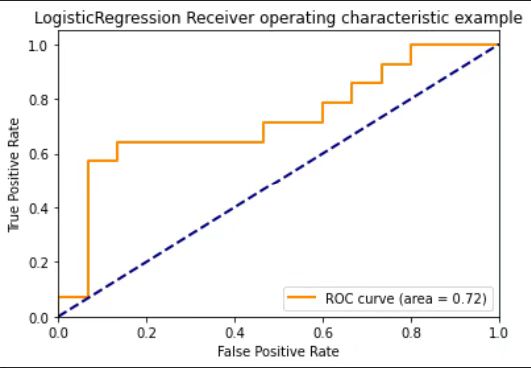
This logistic regression give us an ROC score of 0.72 which is acceptable but definitely has room for improvement.

And other than the count of these five sentiment categories, we also attempt to use the proportion of each category, but the result is not as good as the one we have above, so we do not include it in the blog.
RandomForest
We also try the Random Forest. We understand that this method is not good for finding correlation between variables but we just think it would not hurt to give it a try anyway.
In our example, we split 70% of the data to be training data and the other 30% of the data is used for testing. The train_test_split from sklearn.model_selection is used for splitting.
X_train , X_test , y_train, y_test = train_test_split(X, y_list, train_size = 0.7,shuffle= False)
And for model fitting, RandomForestRegressor from sklearn.ensemble is used.
RFreg = RandomForestRegressor()
RF = RFreg.fit(X_train,y_train)
# predict on training examples
y_predict = RF.predict(X_test)

###compute false positive rate and true positive rate using roc_curve function
fpr, tpr, _ = roc_curve(y_test, y_predict)
roc_auc = auc(fpr, tpr)

###make a plot of roc curve
plt.figure()
lw = 2
plt.plot(fpr, tpr, color='darkorange',
         lw=lw, label='ROC curve (area = %0.2f)' % roc_auc)
plt.plot([0, 1], [0, 1], color='navy', lw=lw, linestyle='--')
plt.xlim([0.0, 1.0])
plt.ylim([0.0, 1.05])
plt.xlabel('False Positive Rate')
plt.ylabel('True Positive Rate')
plt.title('RandomForestRegressor Receiver operating characteristic example')
plt.legend(loc="lower right")
plt.show()
print(roc_auc)
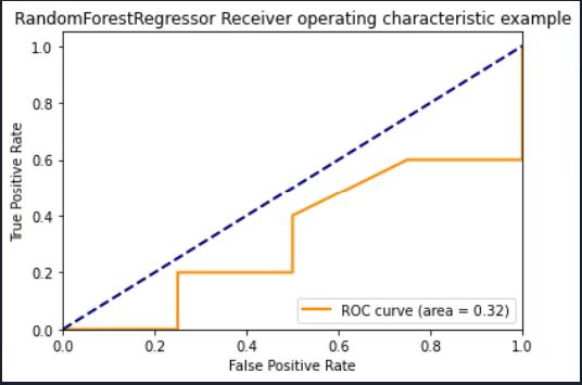
The out-of-sample result from random forest is extremely bad. We only have a 0.32 for ROC. And we have tried other dependent and independent variables but there is no improvement in the result. The reason of this terrible result may be about the small sample size we have. Anyway, it again proves a point that we probably should not use random forest in our case.

Linear Regression
We now come to the simple linear regression. In this case, we take the log transformation of daily close price as y here, and for Xs, we use the daily averaged sentiment score and the count of those five sentiment categories, which we believe could be an indication of bitcoin’s social attention.
d_scoregroupby = d_df.groupby(by=['date']).mean()['Sentiment_Score']
p_df['date']=p_df['Date']
final = pd.merge(p_df,d_scoregroupby , on='date',how = 'right')

final = final.head(29)

final['Close']=final['Close'].apply(lambda x:str(x).replace('$',''))
final['Close']=final['Close'].apply(lambda x:str(x).replace(',',''))
final['Close']=pd.to_numeric(final['Close'])
# data preprocessing to delect the $ and , then change the data type to float

final['logclose'] = np.log(final['Close'])

pivot['SUM'] = pivot['Negative']+pivot['Neutral']+pivot['Strongly Negative']+pivot['Strongly Positive']+pivot['Positive']

final = pd.merge(final,pivot , on='date',how = 'right')

df = final[['Sentiment_Score','SUM']]
LinearRegression from sklearn.linear_model is used to fit the model.
Xtesting = df.iloc[19:29]
Xtraining = df.head(19)
ytraining = final["logclose"][0:19]
ytesting = final["logclose"][19:29]

reg = LinearRegression().fit(Xtraining, ytraining)
model = LinearRegression()
model.fit(Xtraining,ytraining)
r2 = reg.score(Xtraining, ytraining)
The MSE for the model is 0.0011 which seems fine, but the r square value is 0.018 which is surprisingly and extremely low. We will need to explore other variables to obtain a better fit.
LASSO
Last but not least, for LASSO model, for the dependent variable, we use daily close price. And for the independent variables, the five categories for sentiment are used. In this part, we again separate the model into training and testing sets.
Lasso from sklearn.linear_model is used to fit model, and mean_squared_error and mean_absolute_error from sklearn.metrics are used to calculate errors.
train = X[:20]
test = X[-8:]
price = merged

r2_train = []
r2_test = []
mae_train = []
mse_train = []
mae_test = []
mse_test = []

# Perform Lasso
# Define X, Y
x_train = train
y_train = [float(x.replace('$','').replace(',','')) for x in list(price['Close'])][:20]
x_test = test
y_test = [float(x.replace('$','').replace(',','')) for x in list(price['Close'])][-8:]
# Perform Lasso
lasso = Lasso(normalize=True)
lasso.fit(x_train, y_train)
# Get predicted Y
y_train_p = lasso.predict(x_train)
y_test_p = lasso.predict(x_test)
# Get R Square, MAE, MSE
r2_train.append(lasso.score(x_train,y_train))
r2_test.append(lasso.score(x_test,y_test))
mae_train.append(mean_absolute_error(y_train, y_train_p))
mse_train.append(mean_squared_error(y_train, y_train_p))
mae_test.append(mean_absolute_error(y_test, y_test_p))
mse_test.append(mean_squared_error(y_test, y_test_p))
# Collect factors selection frequency

# Prediction error
summary = pd.DataFrame(index = ['In-Sample','Out-of-Sample'])
summary['R Square'] = [sum(r2_train),sum(r2_test)]
summary['MAE'] = [sum(mae_train),sum(mae_test)]
summary['MSE'] = [sum(mse_train),sum(mse_test)]

#summary_avg = summary/len(stockid)# Averaged by all stock ids
Compared with the result from the linear regression model before, the in-sample R square improves a lot reaching 0.5414. However, the out-of-sample R square being negative is very weird which we have to take a closer look into.
Conclusion
To conclude, for now, we can say that the sentiment is somehow correlated with the price change. Among all three models we fit, in terms of r square, Lasso Regression seems to out compete the other two models, but the problem here is that the mechanism of Lasso Regression seems to deviate from the feature of our dataset and the purpose of our project. LASSO is usually used to shrink the number of coefficients to make variable selection. However, we don’t have many variables for our dataset.
All in all, strictly speaking, these models all need to be further improved to achieve better results. And we still need to explore more data variables and try more models to define a specific relationship of what we want to explore. We will discuss other possible flaws in our later challenge part.
