By Group "SenseText"
In this blog, we will mainly focus on the parameter selection of the dimensionality reduction and clustering model. We have explored many possible parameters through loops and visualized the results to select the most suitable configurations.
Dimensionality Reduction
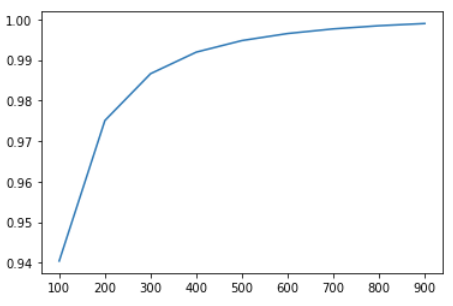
We use PCA for dimensionality reduction. To determine the final number of the dimensions, we print the Dimension – Accumulated-Explained-Variance-Ratio curve:
 |
|---|
| Dimension-Accumulated-Explained-Variance-Ratio Curve |
 |
|---|
| Dimension-Accumulated-Explained-Variance-Ratio Table |
Then we found that a dimension of 300 is good enough to achieve an accumulated explained-variance-ratio of nearly 99%. Increasing the dimension further would not yield a significant improvement. Therefore, we chose 300 as the optimal number of the PCA components.
DBSCAN Clustering
To get the optimal parameters, we explored a range of possibilities by using two loops: for the eps (radius), we tried the threshold [50,150] with an increment of 5; for the minimum ticker sample, we set the value in [4,8] with an increase of 2 in each step. Part of the results are shown in the following table:
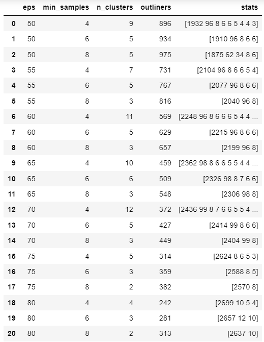
From the result, we found that over 10% of the training companies are always considered outliers. Moreover, the size of the first cluster is out of proportion, containing more than 50% of the companies. Since the resulting clusters are not balanced, this method is not suitable for our project.
SOM Clustering
For this method, cluster sizes were tried form 64 to 144. We found 144 to be the most suitable one. The final model parameters are as follows: clustering size = 144, sigma = 5, learning rate = 0.5, neighborhood function = gaussian.
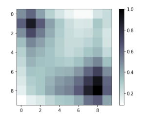
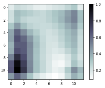
Two of the clustering-density heat maps are as follows:
 |
 |
|---|---|
| cluster size = 100 | cluster size = 144 |
While the 100-cluster case has two concentrated clusters, the 144-cluster case is more dispersed.
K-Means Clustering
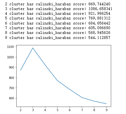
To determine the optimal number of clusters, we first tried Calinski_harabaz score, and found that the optimal cluster size is 3. However, taking data size into consideration, if the number of clusters is 3, each cluster will have almost 1,000 tickers on average, which is unreasonable.
Then we tried the SSE method. We plotted SSE against the number of clusters.
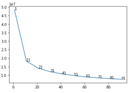
From the curve, we found that SSE improves marginally beyond 51 clusters. To facilitate the comparison with the SOM method, we set 144 as the number of clusters.