By Group "NLP_0"

Introduction

We will build the word matrix based on 10-K files, and use clustering algorithm to count every firm's degree of competition. There are various clustering algorithm and we focus on KMeans and Hierarchical clustering algorithm because these two are popular and easy to understand. The whole process contains three parts: 1. Build the word matrix 2. Conduct clustering with KMeans and Hierarchical clustering algorithm 3. Result and Comparison

Build the word matrix

Thanks to the efforts of our team, we have got the list of processed nouns for every firm every year, and now we decide to build a word matrix for every year based on TFIDF algorithm. The code we use is as follows:

from sklearn.feature_extraction.text import TfidfVectorizer

v = TfidfVectorizer(max_df=0.98,min_df=0.02)#remove the top and bottom 2%

v.fit_transform(word_lst)
word_vector=v.get_feature_names_out().tolist()#word vector

word_matrix=v.transform(word_lst).toarray()#word matrix

Conduct clustering

We decide to cluster all the firms in one year, with about 5000 firms, into 300 groups so that it is meaningful to compare our clustering with the existing industry classification like SIC.

KMeans

K-means clustering is one of the simplest and popular unsupervised machine learning algorithms. K-means algorithm starts with a first group of randomly selected centroids, which are used as the beginning points for every cluster, and then performs iterative (repetitive) calculations to optimize the positions of the centroids until the centroids have stabilized

The code we use is as follows:

from sklearn.cluster import KMeans
import sklearn.metrics

kmeans_model = KMeans(n_clusters=300, random_state=1).fit(result_matrix)
labels = kmeans_model.labels_

Here labels mean the label of cluster that the firm(ie. the vector) is assigned with.

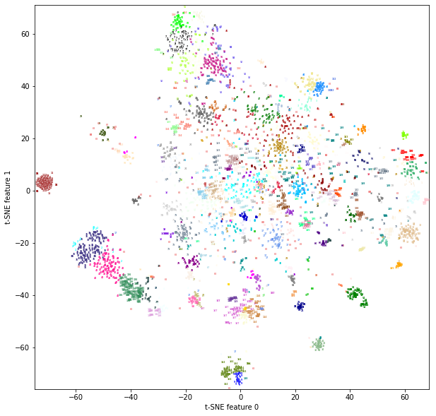
Because the word vector is of high dimension, usually with 2000-3000 dimensions, it is hard to visualize the clustering. Thus, we use TSNE algorithm to reduce dimensionality to two dimensions.

from sklearn.manifold import TSNE
tsne = TSNE(random_state=42)
result_tsne = tsne.fit_transform(word_matrix)

Now we get a two-dimensional matrix and we can use matplotlib to present the clustering effect

import matplotlib.pyplot as plt
import matplotlib.colors as mcolors
mcolor_list = list(mcolors.CSS4_COLORS.keys())[:50] # only present 50 colors
colors = [value for (key, value) in mcolors.CSS4_COLORS.items() 
          if key in mcolor_list]
plt.figure(figsize=(10, 10))
plt.xlim(result_tsne[:, 0].min(), result_tsne[:, 0].max()+1)
plt.ylim(result_tsne[:, 1].min(), result_tsne[:, 1].max()+1)
for i in range(result_matrix.shape[0]):
    plt.text(result_tsne[i, 0], result_tsne[i, 1], 
             str(kmeans_model.labels_[i]),
             color = colors[kmeans_model.labels_[i]],
             fontdict={'weight': 'bold', 'size': 3})
plt.xlabel('t-SNE feature 0')
plt.ylabel('t-SNE feature 1')

The Effect of KMeans Clustering:

Hierarchical clustering algorithm

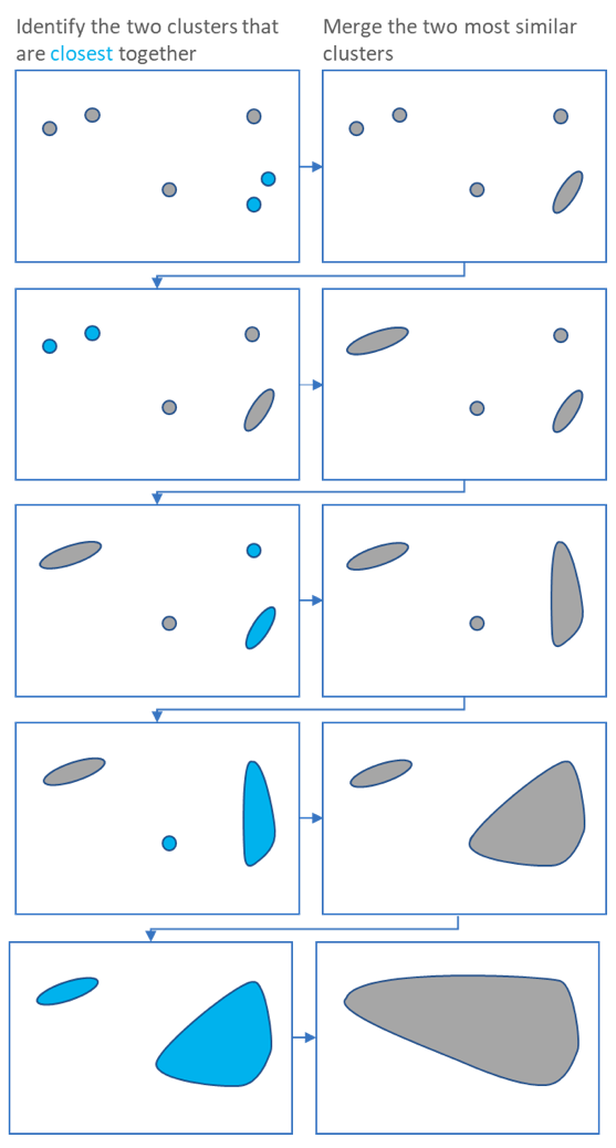
Compared with KMeans, Hierarchical clustering algorithm is more like a bottom-up clustering algorithm. Hierarchical clustering starts by treating each observation as a separate cluster. Then, it repeatedly executes the following two steps: (1) identify the two clusters that are closest together; (2) merge the two most similar clusters. This iterative process continues until all the clusters are merged together. This process is illustrated in the diagrams below.

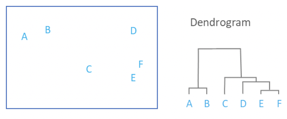
The code we use is as follows:

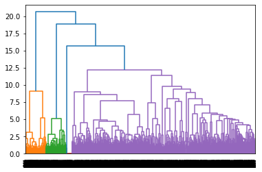
from scipy.cluster.hierarchy import dendrogram, ward
linkage_array = ward(result_matrix)
dendrogram(linkage_array)

# similar algo using sklearn
from sklearn.cluster import AgglomerativeClustering
from collections import Counter
agg = AgglomerativeClustering(n_clusters=300)
assignment = agg.fit_predict(result_matrix)
c = Counter(assignment)
plt.figure(figsize=(10, 7))
plt.bar(x=[str(x) for x in list(c.keys())], height=list(c.values()))
plt.xlabel("assigned labels")
plt.ylabel("# of companies in cluster")
plt.title("300 clusters using AgglomerativeClustering")

And such clustering results can easily be visualized.

Result and Comparison

Because both clustering algorithms are unsupervised learning, it is hard to evaluate their metrics. We import Silhouette Coefficient to help us.

Silhouette Coefficient

The Silhouette Coefficient is defined for each sample and is composed of two scores, and a higher Silhouette Coefficient score relates to a model with better defined clusters. The score is bounded between -1 for incorrect clustering and +1 for highly dense clustering. Scores around zero indicate overlapping clusters. The score is higher when clusters are dense and well separated, which relates to a standard concept of a cluster.

Comparison

We compute the Silhouette Coefficient for both KMeans and Hierarchical clustering algorithm. The result is illustrated below.

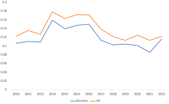
It is obvious that Hierarchical clustering algorithm is better than KMeans here.