By Group "Processors"

Introduction

We have talked about how we fit regression model with bitcoin price and sentiment of social media related text in our last blog. For this blog, we will continue to explore possible relationship between discussion and bitcoin price. More specifically, we will find the buzzwords in the past one month from both social media and news and relate the frequency of these words with the bitcoin price.

The agenda of this blog will be as follow:

1. Finding the Buzzwords
2. Words Selection
3. Model Fitting (News Articles)
4. Model Fitting (Social Media Discussions)

Finding the Buzzwords

Recall that we have gone over the text preprocessing in our past blog. We now can utilize the cleaned text to find our buzzwords by calculating the frequency of each word in all text data from last month. We will go through the text data from Cryptonews to better illustrate the steps.

CountVectorizer from the machine learning module sklearn.feature_extraction.text will be used to calculate the term frequancy. It will generate a table of the frequency of each term in each article. We will then group all articles from the same date and get the daily term frequency.

# each cleaned article becomes one item in the list
text_clean_list = df['text_clean'].to_list()
# count the frequency
count = CountVectorizer()
word_count = count.fit_transform(text_clean_list)
word_count.shape #(150, 6911) -> 150 articles, 6911 unique words
# save in a dataframe and group by date
df_tf = pd.DataFrame(word_count.toarray(), columns = count.get_feature_names())
df_tf = pd.concat([df['Date'], df_tf], axis = 1)
df_tf1 = df_tf.groupby(by = 'Date').sum()
df_tf1.to_csv(os.path.join(file_path, 'cryptonews word count.csv'))

Our definition of buzzwords is the 100 most frequently used words in the text data from the past month. We identify these words by adding up their sum of the daily counts and sort the sum in descending order. We will only keep the top 100 words.

cryptonews_count = df_tf1.T
cryptonews_count['sum'] = cryptonews_count.sum(axis = 1) # get the sum of the frequency count
cryptonews_count['sum'][0] = 10000000 # this is the 'Date' column
cryptonews_count.sort_values(by = ['sum'], ascending = False, inplace = True)
cryptonews_count = cryptonews_count.iloc[0:101] # 100 words + Date
cryptonews_count = cryptonews_count.T
cryptonews_count = cryptonews_count.iloc[0:31] # exclude the sum row

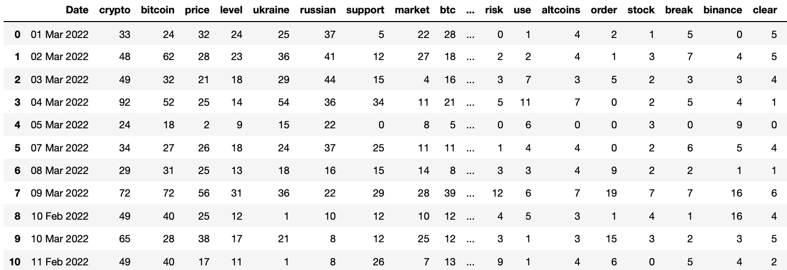
Once we finish the above process, we will a dataframe like this:

Words Selection

Before we fit the frequency of these 100 words with the bitcoin price, we have to manually go through these words to see if they actually make sense. For this part, we just need to use our common sense to consider if a word would be somehow connected to the bitcoin price. For example, for word like "people", I really do not see how it would truly connect to stock price even it may show up in our text data very frequently. This manual selection is very crucial since some uncorrelated words may be very significant in the model but it can just be pure coincidence and our computers will never notice.

delete_list = ['year', 'new', 'news', 'include', 'start', 'announce', 'use', 'total', 'expect', 'people', 'come', 'add', 'level', 'claim', 'clear', 'follow', 'learn', 'price', 'report', 'major', 'country', 'zone', 'market', 'support', 'plan', 'remain', 'high', 'decline', 'break', 'increase', 'accord']
cryptonews_count = cryptonews_count.drop(delete_list, axis = 1)

Another thing we need to do is to combine the count of some words into one. For instance, the word 'ethereum' means the same thing as 'eth' and they should not be treated as two different words. Same thing go with 'russia' and 'russian', 'bitcoin' and 'btc', etc.

cryptonews_count['bitcoin'] = cryptonews_count['bitcoin'] + cryptonews_count['btc'] 
del cryptonews_count['btc']
cryptonews_count['ethereum'] = cryptonews_count['ethereum'] + cryptonews_count['eth']
del cryptonews_count['eth']
cryptonews_count['russia'] = cryptonews_count['russia'] + cryptonews_count['russian']
del cryptonews_count['russian']
cryptonews_count['ukraine'] = cryptonews_count['ukraine'] + cryptonews_count['ukrainian']
del cryptonews_count['ukrainian']

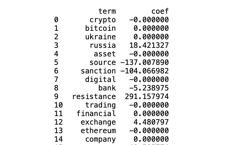
After we are done with manual selection, we can start the automatic selection process where we filter out the statistical insignificant words. We first use LASSO and Ridge (will both be covered in later section) separately to run a regression on all terms passed manual selection. These two methods are very popular for variables selection and regularization. They will shrink the insignificant variables by making their coefficients to or close to zero. Therefore, we will simply select the variables that have non-zero coefficients. A sample result of LASSO is shown below.

Other than LASSO and Ridge, we will also select words using linear regression (will also be covered later). To do that, we will fit the term frequencies with the bitcoin price and look at the summary table of the model.

For the summary table, we will focus on the p-value of each factor other than the constant term. The smaller the p-value is, the more statistical significant the factor will be. However, it will be kind of difficult to determine the cutoff line for small and different people have different belief about that. Yet, we can tell when the p-value is too large, for example, if it is greater than 0.5, so we will eliminate the words with p-value greater than 0.5.

Above is the simplified version of steps we take to narrow down to a list of around 20 words for later model fitting. In the actual selection process, we would have to go back and forth between different models to test and remove one or few terms at a time until we get a satisfying list of words. It is not as straightforward as shown in the above steps since some words can be totally insignificant in one model and very significant in the other. We will just need the best judgement we can when encountering situation like that.

Model Fitting (News Articles)

In this part, we finally start to explore the relationship between bitcoin price and the term frequency of these words. For dependent variable (y), we will use the bitcoin price or its transformation, while for independent variables (X), we will use the term frequency count of each word.

The following models will be covered:

1. Logistic Regression
2. LASSO
3. Ridge
4. Linear Regression

To have a clear idea about the performance of our models, we will split the dataset into training set and testing set during the procedure. We typically use the first 20 days as training and the rest as testing.

Logistic Regression

Logistic Regression is normally used to predict a binary outcome given other observation, thus, its input dependent variable has to be a binary variable. Recall from our last blog, we would indicate the movement of bitcoin price with 0 being going up and 1 being going down. This movement tag will be used as our dependent variable for the model fitting.

Logit from statsmodels.api module will be used to fit the model.

def Logistic_fit(x, y, train_size):    
    x = x.astype(float)

    # splitting the sample into training and testing    
    Xtraining = x[:train_size]
    Xtesting = x[train_size:]
    price = y
    ytraining = price[:train_size]
    ytesting = price[train_size:]

    # Logistic Regression
    lr_model = sm.Logit(ytraining,sm.add_constant(Xtraining)).fit()
    print(lr_model.summary()) # get a summary result

    # get the prediction
    predicted_prob = lr_model.predict(sm.add_constant(Xtraining))

    #compute false positive rate and true positive rate using roc_curve function
    fpr, tpr, _ = roc_curve(ytraining, predicted_prob)
    roc_auc = auc(fpr, tpr)

    # testing
    predicted_prob1 = lr_model.predict(sm.add_constant(Xtesting))
    fpr, tpr, _ = roc_curve(ytesting, predicted_prob1)
    roc_auc = auc(fpr, tpr)

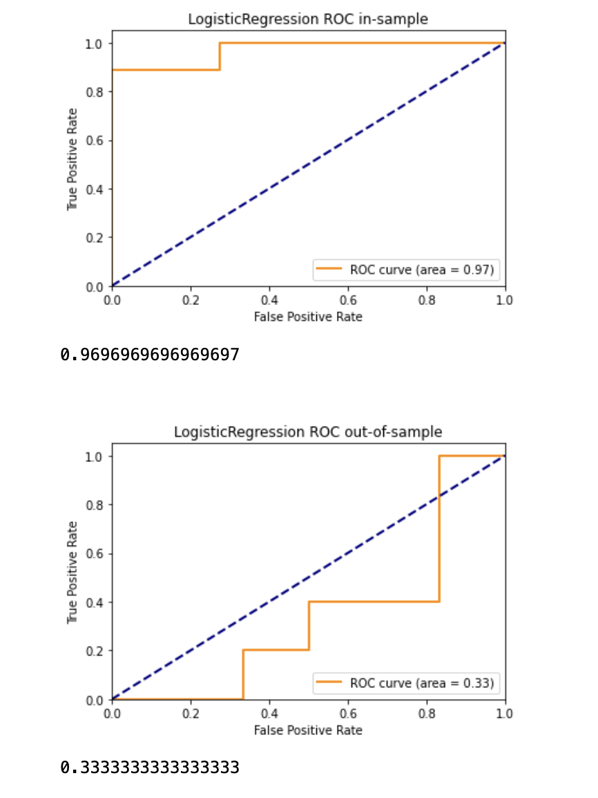
The below result is obtained. The in-sample AUC is 0.97 while the out-of-sample ROC is 0.33. The Pseudo R^2 for this model is 0.6428.

LASSO

Unlike we only have five sentiment categories as independent variables last time, we have many term frequency variables this time which makes it a good dataset for LASSO regression. LASSO will automatically select the useful variables and discard the insignificant ones.

For this model, the price will be used as the dependent variables. We will useLasso from sklearn.linear_model to fit the model. And we will calculate the error using mean_squared_error and mean_absolute_error from sklearn.metrics.

def LASSO_fit(x, y, train_size):
    # separate training and testing
    train = x[:train_size]
    test = x[train_size:]
    price = y

    r2_train, r2_test = [], []
    mse_train, mse_test= [], []
    mae_train, mae_test= [], []

    # Define X, Y 
    x_train = train
    y_train = price[:train_size]
    x_test = test
    y_test = price[train_size:]

    # Perform Lasso
    lasso = Lasso(normalize=True)
    lasso.fit(x_train, y_train)

    # Get predicted Y
    y_train_p = lasso.predict(x_train)
    y_test_p = lasso.predict(x_test)
    # Get R Square, MAE, MSE
    r2_train.append(lasso.score(x_train,y_train)) 
    r2_test.append(lasso.score(x_test,y_test)) 
    mae_train.append(mean_absolute_error(y_train, y_train_p))  
    mse_train.append(mean_squared_error(y_train, y_train_p)) 
    mae_test.append(mean_absolute_error(y_test, y_test_p))  
    mse_test.append(mean_squared_error(y_test, y_test_p))  

    # Prediction error
    summary = pd.DataFrame(index = ['In-Sample','Out-of-Sample'])
    summary['R Square'] = [sum(r2_train),sum(r2_test)]
    summary['MAE'] = [sum(mae_train),sum(mae_test)]
    summary['MSE'] = [sum(mse_train),sum(mse_test)]

The result of the LASSO regression is shown below.

Ridge

Ridge is very similar to LASSO, except that LASSO will reduce some coefficients to zero as compared to Ridge which never sets any to zero but only brings them to very close to zero.

Ridge from sklearn.linear_model will be used in the code below. Since we input the same variables as we do in LASSO and the code of Ridge is very similar to that for LASSO, we will only show the part of the code that is different.

def Ridge_fit(x, y, train_size):
    # the first part is exactly the same as LASSO so we won't show it here

    # Perform Lasso
    ridge = Ridge(normalize=True)
    ridge.fit(x_train, y_train)

    # Get predicted Y
    y_train_p = ridge.predict(x_train)
    y_test_p = ridge.predict(x_test)

    # Get R Square, MAE, MSE
    r2_train.append(ridge.score(x_train,y_train)) 
    r2_test.append(ridge.score(x_test,y_test)) 
    mae_train.append(mean_absolute_error(y_train, y_train_p))  
    mse_train.append(mean_squared_error(y_train, y_train_p)) 
    mae_test.append(mean_absolute_error(y_test, y_test_p))  
    mse_test.append(mean_squared_error(y_test, y_test_p))

The result from Ridge is also very similar to that from LASSO.

Linear Regression

For the classic linear regression, we try to use the price to be the dependent variable but it seems like the log transformation of the price gives a better result so we use the log price instead.

OLS from statsmodels.api will be used to perform the regression.

def Linear_fit1(x, y, train_size):    
    x = x.astype(float)

    # splitting the sample into training and testing    
    Xtraining = x[:train_size]
    Xtesting = x[train_size:]
    price = y
    ytraining = price[:train_size]
    ytesting = price[train_size:]

    # fit OLS
    reg = OLS(ytraining,sm.add_constant(Xtraining)).fit()
    #result = reg.fit_regularized(alpha=2., L1_wt=0, refit=True)

    print(reg.summary())

     # out of sample  
    yhat_train = reg.predict(sm.add_constant(Xtraining))
    yhat_test = reg.predict(sm.add_constant(Xtesting))    

    # MSE and r2
    MSE_in = reg.mse_model
    MSE_out = metrics.mean_squared_error(ytesting,yhat_test)
    r2_in = reg.rsquared
    #r2_out = ytesting.corr(yhat_test)**2
    var_test = np.var(ytesting)
    r2_out = 1-MSE_out/var_test

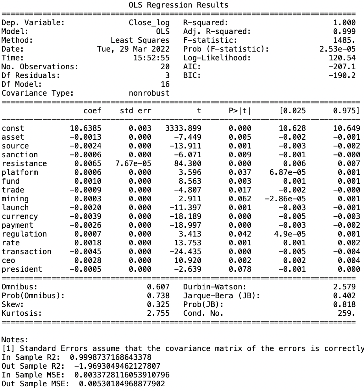
The result of linear regression is shown below. We obtain a R^2 of 1.

Model Fitting (Social Media)

With Term Frequency

As for discussions on social media (Bitcointalk,Yahoo Finance Community, Reddit, and Twitter), we decide to sum up the word count for each word from the four platforms in terms of date, and get the top 100 terms with the highest frequency. Since the data from different platforms ranges in different dates, we only choose data from February 16 to March 16.

df = twitter_dic.groupby('Date').sum().add(yahoo_dic.groupby('Date').sum(), fill_value=0).add(bitcointalk_dic.groupby('Date').sum(), fill_value=0).add(reddit_dic.groupby('Date').sum(), fill_value=0)
to_be_customized = df.iloc[46:75,:].sum().sort_values(ascending = False).head(n = 200)  # df.iloc is for date selection

Similar with model fitting with news articles, we fit the 100 terms from social media in the four models and manually delete words from the top 100 based on the performance, reaching to a list of around 1o words.

 for term in list(to_be_customized.index):
    if term in delete_list:
        del to_be_customized[term]
len(list(to_be_customized.index))

# Final Term List
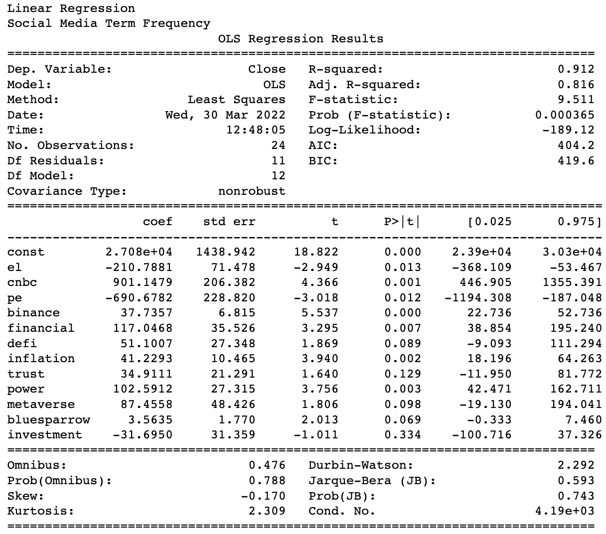
term_list = ['el','cnbc','pe','binance','financial','defi','inflation','trust','power','metaverse','bluesparrow','investment']

The final result of linear regression OLS is as below.

With Term Frequency and Sentiment

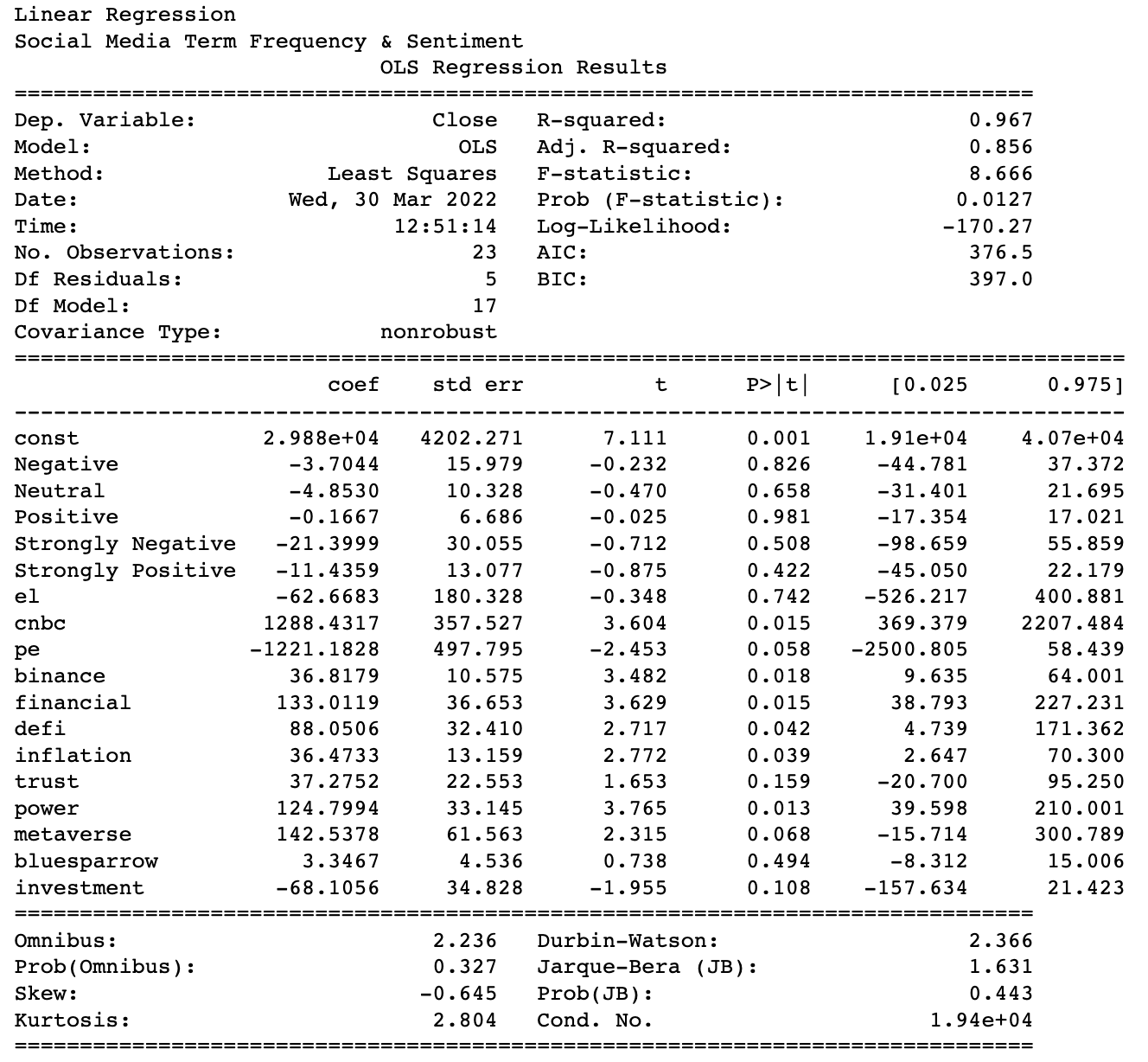
To explore futher relationships, we also fit the selected term frequencies in the four models again together with the total counts of five sentiment categories. In addition, we make the sentiment counts go through the models alone for comparison.

df_sen = twitter_sen.groupby('Date').sum().add(yahoo_sen.groupby('Date').sum(), fill_value=0).add(bitcointalk_sen.groupby('Date').sum(), fill_value=0).add(reddit_sen.groupby('Date').sum(), fill_value=0).reset_index()
df = pd.merge(df_sen, term_df, on = 'Date', how = 'right')

The final result of linear regression OLS is as below.

Final Analysis

We will provide further analysis on the models and the outputs in our report.