By Group "Tower of Babel"
After capturing the data we need, we promoted our project as the following steps:
-
Data cleaning
-
Text Processing
-
Analysis & Visualization
1. Data cleaning
The data we captured from the website contains so much redundancy that we do not need. Therefore, in this section, I would record the obstacles we encountered and what we did to transform the raw data into the format we can use.
The most important data we need is the information in the column ‘review_revs’ which contains the content of the reviews. However, there are some reviews are written in non-English language that can so we need to delete them.
The most important data we need is the information in the column ‘review_revs’ which contains the content of the comment. However, there are some comments are written in non-English language so we need to delete them. Every non-English comment is end with ‘Translate review to English’, therefore we only need to keep comments without this sentence:
dg = dg.loc[~dg['review_revs'].str.contains('Translate review to English')].copy()
There are some not-real-review information at the end of each comment that need to be deleted, for example ‘Helpful’, ‘Report abuse’.
destr = "found this helpful', 'Helpful', 'Report abuse'"
destr2 = "'Helpful', 'Report abuse'"

item = list(dg['review_revs'])
a_list = []
for i in item:
    i = i.replace(destr,'')
    i = i.replace(destr2, '')
    a_list.append(i)
dg['review_revs'] = a_list
2. Text Processing
In this section, I would introduce the main steps of text processing in our project.
Step 1. Convert all the text into lowercase
df['review'] = df.review.apply(lambda x: x.lower())
Step 2. Remove punctuation
punctuation_str = string.punctuation
df['review'] = df.review.apply(lambda x: re.sub(r'[{}]+'.format(punctuation_str),"",x))
Step 3. Remove stopwords & Tokenize
Stopwords generally don’t convey much valuable information but can frequently appear in the text. Removing stopwords can increase efficiency and accuracy of text analysis.
We download 'stopwords' by 'nltk' :
import nltk
import ssl

try:
    _create_unverified_https_context = ssl._create_unverified_context
except AttributeError:
    pass
else:
    ssl._create_default_https_context = _create_unverified_https_context

nltk.download('stopwords')
And then, use module 're' to do the tokenize (for we can not successfully download the package 'tokenize'):
alist = df['review'].tolist()
blist = []
clist = []
stopw = stopwords.words('english')

for id in alist:
    #delete numbers
    cc = re.sub(r'[0-9]',"",id)
    x=0
    #delete stopwords
    while x<len(stopw):
        cc = cc.replace(' '+stopw[x]+' '," ")
        #cc = cc.replace(stopw[x]+' '," ")
        x+=1
    bb = list(filter(None,cc.split(" ")))
    blist.append(bb)
    clist.append(cc)

df['review_tk'] = blist

df['review_untk'] = clist
3. Analysis & Visualization
In this section, we mainly use packages 'seanborn', 'wordcloud' and 'matplotlib' to visualize our results.
1) Ratings for overall and different models
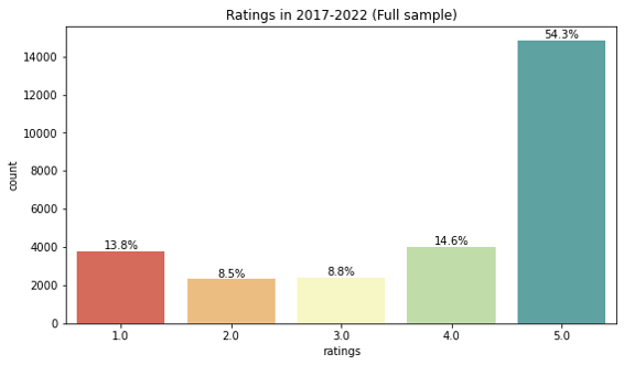
We want to get the percentage of different scores (1,2,3,4,5) , so we define the function rate(input_data,name) to show the frequency of each score in one histogram.
input_data should be a DataFrame,
name should be a string:
def rate(input_data,name):
    fig = plt.figure(figsize=(9,5))
    ax = sns.countplot('review_stars',data=input_data,palette='Spectral')
    plt.xlabel('ratings')
    plt.title('Ratings in 2017-2022 ({})'.format(name))

    # show the frequency in the histogram
    ncount = len(input_data)
    for p in ax.patches:
        x=p.get_bbox().get_points()[:,0]
        y=p.get_bbox().get_points()[1,1]
        ax.annotate('{:.1f}%'.format(100.*y/ncount), (x.mean(), y),
                ha='center', va='bottom') # set the alignment of the text
    plt.show()
Then we call the function to get the score percentage of holistic data:
rate(df,'Full sample')
Here is the result:

Above is an example, it is almost the same if we want to get the score percentage of a specific model, the only difference is that we need to filter the specific rows from the whole dataframe before we call the function:
data_1 = df[df['asin'].isin(['B07D75MVX9'])].copy()
and then, call the function. Please pay attention to the 'input_data', changes from 'df' to the dataframe that we get from last line:
rate(data_1,'Eufy 30C')
2) Key words of 5-score reviews in different models
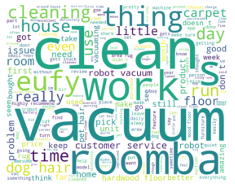
We want to know the key words of high-rated comments, so we decide to find 14 words that most frequently appeared in the 5-score comments.
First, pick out all the 5-score comments:
key_words = df[df['review_stars']==5]['review_untk'].values
Second, split all the 5-score comments into single words and save in a list:
words_list=[]
for word in key_words:
    l = word.split(' ')
    for i in l:
        words_list.append(i)
Third, exclude some general good words such as 'good', 'great', 'like', 'love':
de_list = ['one','get','every','love','great','much','like','well','would','job']
stopw_1 = stopw.copy()
stopw_1.extend(de_list)
words_list_1 = [w for w in words_list if not w in stopw_1]
Forth, visualize the result using wordcloud:
words = ','.join(words_list_1)
wordcloud = WordCloud(background_color='white',width=1000,height=800).generate(words)
plt.imshow(wordcloud, interpolation="bilinear")
plt.axis("off")
plt.show()
Here is the wordcloud result:

In addition to the high-score wordcloud, we also made a low-score wordcloud. The process is almost the same except that we have to exclude some general bad words rather than good.
3) Vader Emotion Score of different models
We grade all the comments according to their emotion tendency by using 'Vader':
from vaderSentiment.vaderSentiment import SentimentIntensityAnalyzer
sentences = list(df['review_revs'])
analyzer = SentimentIntensityAnalyzer()
scores = []
for sentence in sentences:
    vs = analyzer.polarity_scores(sentence)
    scores.append(vs['compound'])
df['scores_Vader'] = scores
And plot the result of emotion score into a line chart.
Above is the basic structure and also the idea that we followed when we develop our code. Hope this will help with going through our code.