By Group "Money Maker"
Introduction and Objectives
In the case of information overload, the rapid use and mining of information asymmetry has become the focus of competition among all kinds of financial asset management institutions in the era of big data.
Following the trend in NLP, our group project focused on analyzing and comparing two different sources of text information:
- We chose the famous news website Barron's to get the past two year data of the news headlines about Tesla. At the beginning, the website we chose was scrolling, but we found it difficult to implement the scrolling code, so we chose Barron's.
- The tweets from the social media platform Stocktwits about Tesla. Since Barron's data is relatively small, we have added stocktwits to enrich the content.
With the support of information scraped, we mainly used two helpful methods in predicting market and analyzing the feasibility:
- Classification Prediction
- Sentiment Analysis
Then, we compared the sentiment scores with the fluctuation of stock price, afterwards analyzed the correlation between two different resources and explained why correlation exits different.
Date Processing
Firstly, we should do some web-scraping and data-cleaning as a cornerstone for NLP technology.
In the web-scraping process, we have scraped the news headlines in the past 2 years after considering the headlines can completely illustrate significant information.
def crawler(page):
df = pd.DataFrame()
browser = webdriver.Chrome(executable_path = driver_path)
for i in range(31,page+1):
print(i)
df0 = pd.DataFrame()
url = 'https://www.barrons.com/search?query=tesla"equery=tsla&mod=DNH_S&page=' + str(i)
browser.get(url)
titles = browser.find_elements_by_xpath('//*[@id="root"]/div/div/div/div[2]/div/div/div[4]/article[position()>=1]/div[1]/div[2]/h4/a/span')
title_lst = pd.Series(list(map(lambda x: x.text, titles)))
times = browser.find_elements_by_xpath('//*[@id="root"]/div/div/div/div[2]/div/div/div[4]/article[position()>=1]/div[1]/div[3]/div/p')
time_lst = pd.Series(list(map(lambda x: x.text, times)))
df0['Date'] = time_lst
df0['News'] = title_lst
print(len(df0))
df = pd.concat([df,df0],ignore_index=True)
time.sleep(1)
browser.quit()
return df
The process for scraping information is different with Barron, we used API key to directly scrape comments from Stocktwits and information were saved as jsom form automatically through this method.
The time spent on Stocktwits web-scraping were time-consuming and it took almost 3 days to finish.
def stocktwits_json_to_df(data, verbose=False):
    #data = json.loads(results)
    columns = ['id','created_at','username','name','user_id','body','basic_sentiment']
    db = pd.DataFrame(index=range(len(data)),columns=columns)
    for i, message in enumerate(data):
        db.loc[i,'id'] = message['id']
        db.loc[i,'created_at'] = message['created_at']
        db.loc[i,'username'] = message['user']['username']
        db.loc[i,'name'] = message['user']['name']
        db.loc[i,'user_id'] = message['user']['id']
        db.loc[i,'body'] = message['body']
        #We'll classify bullish as +1 and bearish as -1 to make it ready for classification training
        try:
            if (message['entities']['sentiment']['basic'] == 'Bullish'):
                db.loc[i,'basic_sentiment'] = 1
            elif (message['entities']['sentiment']['basic'] == 'Bearish'):
                db.loc[i,'basic_sentiment'] = -1
            else:
                db.loc[i,'basic_sentiment'] = 0
        except:
                db.loc[i,'basic_sentiment'] = 0
        #db.loc[i,'reshare_count'] = message['reshares']['reshared_count']
        for j, symbol in enumerate(message['symbols']):
                db.loc[i,'symbol'+str(j)] = symbol['symbol']
        if verbose:
            #print message
            print(db.loc[i,:])
    db['created_at'] = pd.to_datetime(db['created_at'])
    return db
After collecting more than enough textual data, we had to do data cleaning and preparing for LDA technology and other process. Under the form of all English words, we used WordNetLemmatizer from nltk.stem.wordnetl in order to respond uniformly to different spellings of the same semantic root and lemmatized them.
from nltk.corpus import stopwords
from nltk.stem.wordnet import WordNetLemmatizer
import string

stop = set(stopwords.words('english'))
pat_letter = re.compile(r'[^a-zA-Z]+')
lemma = WordNetLemmatizer()

def clean(text):
    stop_free = " ".join([i for i in text.lower().split() if i not in stop])
    punc_free = re.sub(pat_letter," ",stop_free)
    short_free = " ".join([w for w in punc_free.split() if len(w)>2])
    normalized = " ".join(lemma.lemmatize(word) for word in short_free.split())
    return normalized

tesla['clean'] = tesla['News'].apply(lambda x: clean(x).split(' '))
tesla
Stock Price Movement Prediction
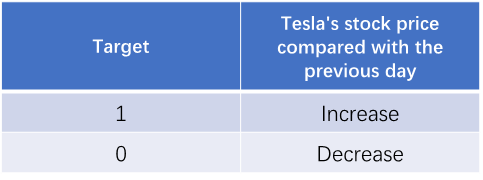
Firstly, we created the target variable using Tesla’s stock price. The target is ‘1’ if the close price of that day rise compared to the previous day, ‘0’ if the close price decrease compared to the previous day.
Then we selected 7 different classification models as our candidates, which are Logistic Regression, Naïve bayes, KNN, SVM, Random Forest, Extra Trees, AdaBoost. These models are all classic models that usually work well in filtering baseline models.
Now only use Naive Bayes as an example
from sklearn import naive_bayes, svm, neighbors, ensemble
from sklearn.metrics import confusion_matrix, accuracy_score, f1_score
from sklearn.linear_model import LogisticRegression

lr_model = LogisticRegression()
nb_model = naive_bayes.GaussianNB()
knn_model = neighbors.KNeighborsClassifier()
svc_model = svm.SVC(probability=True, gamma="scale")
rf_model = ensemble.RandomForestClassifier(n_estimators=100)
et_model = ensemble.ExtraTreesClassifier(n_estimators=100)
ada_model = ensemble.AdaBoostClassifier()

models = ["lr_model", "nb_model", "knn_model", "svc_model", "rf_model", "et_model", "ada_model"]

def baseline_model_filter(modellist, X, y):
    X_train, X_test, y_train, y_test = train_test_split(X, y, test_size = 0.3, random_state = 200)
    for model_name in modellist:
        curr_model = eval(model_name)
        curr_model.fit(X_train, y_train)
        y_pred = curr_model.predict(X_test)
        print(f'{model_name} \n accuracy:{accuracy_score(y_test, y_pred)}\n f1 score:{f1_score(y_test, y_pred)}\n confusion matrix:{confusion_matrix(y_test, y_pred)}')

baseline_model_filter(models, X, y)
The ultimate results are as follows.
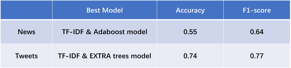
According to the results, we get to conclude that both news and tweets can predict the stock price movement to some extent. And tweets have shown a stronger predicting power than the news headlines.
LDA Model and Visualization
The whole LDA topic modeling takes 3 parts:
- Obtained the TF-IDF word frequency matrix through text vectorization
- Trained the LDA topic model on them
- Realize dynamic and static visualization of topic distributions
LDA related codes are as follows:
#LDA-Model
train = tesla['clean']
num_topics = 3
#Build dictionary
dictionary = corpora.Dictionary(train)
V = len(dictionary)
#Construct sparse matrix of texts
corpus = [dictionary.doc2bow(text) for text in train]  # get sparse vector of text
#Caculate TF-IDF weights
corpus_tfidf = models.TfidfModel(corpus)[corpus]
# train LDA model
tesla_lda = models.LdaModel(corpus_tfidf, num_topics=num_topics, id2word=dictionary,
                          alpha=0.01, eta=0.01, minimum_probability=0.001,
                          update_every=1, chunksize=100, passes=1)
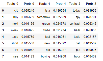
The distribution of topics is shown in the table:
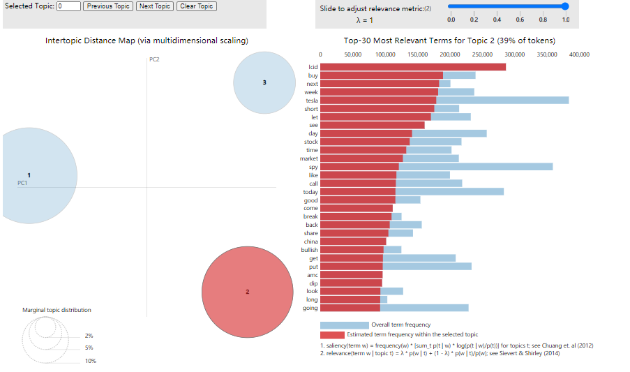
PyLDAvispresents an interactive visualization of the LDA model.
# LDA Model visualization
import pyLDAvis.gensim_models
# Display in notebook by pyLDAvis
plot =pyLDAvis.gensim_models.prepare(tesla_lda,corpus,dictionary)
pyLDAvis.save_html(plot, 'H:/nlp/groups/tesla_lda.html')
The bubbles on the left are for different topics, and the top 30 words on the right are for different topics. Light blue shows the frequency (weight) of the word throughout the document, and dark red shows the weight of the word within the topic.
Sentiment Analysis
In order to quantify the emotions in the text, we chooseTextblob package to help us. Textblob is a package that can give each sentence a sentiment score, which is a number between negative one and positive one. We used this package to give every financial news headline a sentiment score, and then calculated the average score for each single day.
Since the publication date of the news data we collected was from March 19, 2021 to March 20, 2022, we obtained the daily stock history data of all trading days in the same period from Yahoo Finance, including closing price, volatility and return rate. Then we calculated the correlation coefficient between these market data and news sentiment score respectively.
tweets = df['tweet'].tolist()
sentis = []
for item in tweets:
    blob = TextBlob(item)
    senti = blob.sentiment
    sentis.append(senti[0])
df['sentiment'] = sentis
df
The calculation results of correlation coefficient are shown as below
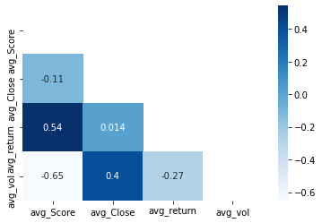
The correlation coefficient between sentiment score and return rate is 0.54. We smoothed the data and draw a chart, which is shown as below:
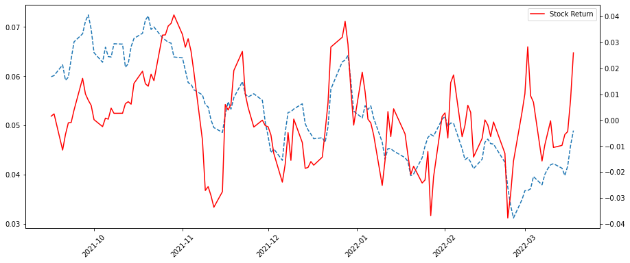
The graph also clearly shows this strong correlation, meaning that the sentiment of tweets is more correlated with the stock market than the sentiment of news.
Summary
Reviewing our team's project, we used financial news and stocktwits texts as data sources, and got three main conclusions: first, financial news mainly focuses on market business activities and competitiveness of products, while tweets focuse on investors’ individual judgement and performance of the whole market; Second, text data can be used to predict the price movement, and tweets did better. Third, there is a correlation and a similar trend between text sentiment and stock’s market performance, and the sentiment of tweets has a stronger correlation.