For this blog post, we will provide a cumulative review and reflection on our project, 'ESG & Volatility,' specifically on the Sentiment Analysis and Stock Volatility portion of our project.
Sentiment Analysis:
Using the cleaned text data, we then conducted sentiment analysis on the news articles by using Vader from NLTK. Our plan was to calculate the sentiment score for each date in order to match them with the daily volatility data later on in our process. Therefore, the articles were sorted into ascending order of dates. However, we realized that the number of news articles that were scraped varied for each date. First, we attempted to summarize the news sentiment of each date by determining the average sentiment score for every article. Below shows the code snippet of our initial attempt:
# Open the cleaned_data CSV file
data = pd.read_csv('final_data.csv')


# Calculate sentiment scores for each article
sentiment_scores = []
dates = []
analyzer = SentimentIntensityAnalyzer()
for index, row in data.iterrows():
   sentiment_score = analyzer.polarity_scores(row['text'])['compound']
   sentiment_scores.append(sentiment_score)
   dates.append(row['date'])


# Create a DataFrame with the dates and sentiment scores
sentiment_data = pd.DataFrame({'date': dates, 'sentiment_score': sentiment_scores})


# Calculate average sentiment scores for each date
average_sentiment_scores = sentiment_data.groupby('date')['sentiment_score'].mean().reset_index()


# Convert date column to datetime format with specified format
average_sentiment_scores['date'] = pd.to_datetime(average_sentiment_scores['date'], format='%m/%d/%y')


# Sort the average sentiment scores DataFrame by date in ascending order
average_sentiment_scores = average_sentiment_scores.sort_values(by='date').reset_index(drop=True)
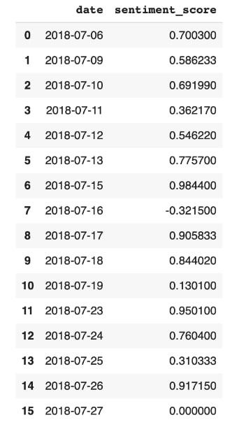
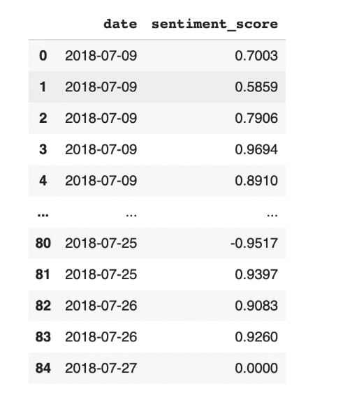
In general, the results showed that most of the positive event articles exhibited positive average sentiment scores, confirming that the event was indeed reflected in the news articles with positive sentiment. However, we acknowledged that the dataset was very limited in size, which was going to make it challenging to obtain reliable results in our regression analysis in the future. Consequently, instead of calculating the average for each date, we decided to calculate the individual sentiment scores from all the articles we had scraped, which provided us with a larger dataset to conduct our regression analysis. Below, we show the initial outcome of the average sentiment scores on the left-hand side, which consists of 16 datasets, and the updated sentiment score calculation on the right-hand side, which consists of 85 datasets. Another important point to mention is that in our first attempt, the date of the first news article was mistakenly recorded as July 6th instead of the correct date, which is July 9th. This happened because when we scraped the articles, some of them failed to process the dates and showed NaN, and we had to manually input the dates ourselves. We discovered this error and successfully incorporated the corrected date in our final version of the sentiment analysis. Then, we calculated the sentiment scores for the negative articles by applying the same method. Overall, the sentiment analysis process provided us with valuable lessons, such as the significance of dataset size and data quality control.
Stock Volatility:
While working on our project, we struggled to determine the best method to calculate and analyze the volatility in the best manner. In the beginning, our team considered using the traditional method of computing the annualized standard deviation of daily returns, which was the conventional approach to calculating volatility. The method was quite simple, but our existing dataset has data that is of a narrow time horizon. After reviewing extensive literature, we concluded that this method is used most of the time to study longer and fixed-time volatility conditions and may not be responsive to short-term sharp fluctuations. In our case, it may not be useful because our project is to capture rapid changes in volatility within a month of a news release.
To address the problem, we turn to the rolling volatility method. This method calculates the standard deviation of returns within a moving window, which is more sensitive to changes, suitable for short-term risk, and more in line with our project objectives.
import yfinance as yf
import pandas as pd
import numpy as np

data = yf.download('SBUX', start='2018-04-01', end='2018-05-01')

data['Returns'] = data['Adj Close'].pct_change()

data['Rolling_Volatility'] = data['Returns'].rolling(window=2).std() * np.sqrt(252)

start_date = '2018-04-16'
end_date = '2018-04-27'

result = data.loc[start_date:end_date, ['Rolling_Volatility']]

result.columns = ['rolling_volatility']

print("Calculated Rolling Volatility:")
print(result)

filename = 'SBUX_Rolling_Volatility_April_2018.csv'
result.to_csv(filename, index_label='date')

read_back_data = pd.read_csv(filename, index_col=0)

print("\nData read from CSV:")
print(read_back_data)
The Python code above showed how we calculated volatility when negative news occurred. We obtained historical stock data of Starbucks (ticker: SBUX) for the month of April 2018 using the “yfinance” library. From this data, daily returns were calculated based on the adjusted closing price of the stock. Then, using the returns, we computed rolling volatility for the 2-day window and then annualized it by multiplying it with the square root of 252 (the normal trading days in a year). We then screened the data by specifically filtering for the date range of April 16, 2018, to April 27, 2018, as this was the actual range of dates when the negative news had occurred. The column names of the generated data frame were then converted into lowercase for consistency. We displayed the rolling volatility of the returned results with a date range saved to the CSV file, “SBUX_Rolling_Volatility_April_2018.csv,” using the “date” column as an index. Lastly, this code read the saved CSV file back into a new data frame. Finally, it read the saved CSV file back into a new data frame to ensure that the data was stored properly and in the right format. Finally, it printed the data to display what it contained.
When computing rolling volatility, we broadened the data range to include more than just the specific period being analyzed. For example, we might collect a full month's worth of stock data, even if our focus is on a shorter timeframe. This approach helps address edge effects by ensuring that calculations at the boundaries of our dataset are not skewed due to insufficient data. This ensures better consistency and accuracy throughout the analysis period and is also a step towards statistical robustness. The "warm-up" period in our model ensures that from the start, the rolling window benefits from a sufficient quantity of data, thus mitigating any potential inaccuracies caused by a limited number of data points. By incorporating a broader dataset, this approach enhances the model's ability to estimate volatility more accurately and stabilizes the impact of market variability.