By Hanna

Text Classification and Information Retrieval

1. What this Post is About:

This blog post serves as some kind of personal documentation of all the problems, the solutions I came across and the learnings, that I experienced along the journey of my final project. In particular, this blog post does neither cover the broader context of the project, nor does it particularly elaborate on the findings, limitations, future work etc.
If the reader is interested in those, he or she is referred to the presentation slides and the report accompanying this project.

2. Background

In this project, my principal goal is to do text classification and information retrieval on text data using two different supervised machine learning models (naive Bayes and logistic regression). As a start, I refer to the Rotten Tomatoes movie dataset, which is a collection of \(45368\) movie reviews, initially collected by Pang and Lee rottentomatoes.com.

Since I am new to natural language processing I find this an adequate data set to start with. I aim to implement two supervised classification models that should be able to classify a movie review as either a positive (\(\rightarrow $ 1) or negative one (\)\rightarrow $ 0) respectively. That is, I will fist try to do binary classification on the data before extending it to multi-class classification. Note that, while I implemented the option to do multi-classification in the file evaluation-metrics.py, the project ultimately remains limited to binary classification. Multi-classification remains subject to future work since I spent the bulk of the time first, understanding the NLP-pipeline, second, learning about feature extraction methods, evaluation metrics and most importantly, classification algorithms in theory, while subsequently spending quite some time implementing them in code.

Side note: I only learned later, that for instance, Bag of Word, which I use for feature extraction, and Naive Bayes and Logistic Regression actually come pre-implemented in some python packages. Since I was not aware of that, I implemented these methods from scratch.

3. Project Architecture

In the following, a brief overview of the project's architecture is given by listing the project's data- and code-files.

Data-files

• train.csv contains the sentences and their associated sentiment labels for training.
• valid.csv contains the sentences and their associated sentiment labels for validation.
• test.csv contains just sentences. The trained model is supposed to assign a label to each sentence.

Code-files

• model.py is the main entry of this project.
• metrics.py contains classification metrics including accuracy, precision, recall, and F-Score.
• feature-extractor.py contains functions to extract features from raw text.
• models.py contains classification algorithms.
• sentiment-data.py contains functions to process raw data.

4. Text Preprocessing

Machine learning models work particularly well on numbers. This is, why we first need to transform our input (Strings) into numbers. We also do some other data processing, such as: - tokenization - converting words into lowercase - removing punctuations - removing stopwords

For this, we import the python package NLTK:

import nltk
from nltk.corpus import stopwords

Then we can define the text_preprocessing method:

def text_preprocessing(sentence: str) -> List[str]:
    """Preprocess text"""
    words = []

    # divide sentence into tokens
    tokens = nltk.word_tokenize(sentence)

    # convert tokens to lowercase
    for t in tokens:
        words.append(t.lower())
    # remove punctuations
    words = [w for w in words if w.isalpha()]

    # remove stopwords
    stop_words = list(stopwords.words("english"))
    words = [w for w in words if w not in stop_words]

    return words

5. Evaluation Metrics

There are many evaluation metrics such as accuracy, precision, recall and ultimately F-Score, which is a combination of the former two. and first, I did not bother about which one to choose, until I learned, that it might be some significant, as to which metric is chosen. The most intuitive metric to me seemed to simply take the accuracy, but more on this you'll find further down the lines. Later I learned the importance of using more refined evaluation metrics, but let's first have a look at the confusion matrix: This is because, prior to being able to evaluate anything, we first need to summarize the predictions that our model has made by basically counting how often it classified inputs correctly or incorrectly. This is done in a confusion matrix (see Figure):

5.1 Confusion Matrix:

In the confusion matrix, \(TP\) denotes the true positives, \(TN\) the true negatives, \(FP\) the refers to the false positives and \(FN\) denotes the false negatives. Then the evaluation metrics can be derived as follows: - #### Accuracy: - Accuracy is a corse metric describing the proportion of correct classifications. In particular, two models may have the same accuracy while behaving very differently. - \(Accuracy = \frac{TP + TN}{\text{Total}}\)

• Precision:
  • Precision(+) describes the proportion of correct positive classifications from cases that are predicted as positive. More generally, it refers to the percentage of selected classes that are correct.
  • \(Precision(+) = \frac{TP}{TP + FP}\)
  • \(Precision(-) = \frac{FN}{FN + TN}\)

• Recall:

  • Recall(+) describes the proportion of correct positive classifications from cases that are actually positive.
  • \(Recall(+) = \frac{TP}{TP + FN}\)
  • \(Recall(-) = \frac{TN}{TN + FP}\)
  • More generally, recall describes the percentage of correct items selected.

With the following command python3.7 metrics.py

----------------------------------------
Test for macro average: 
Accuracy: 0.6220
Precision: 0.4375
recall: 0.4351
F score: 0.4363
----------------------------------------
Test for micro average: 
Accuracy: 0.6220
Precision: 0.6220
recall: 0.6220
F score: 0.6220

For reference, let's compare to the scikitlearn method preisision_recall_fscore_method in metrics:

(0.4375311399504369, 0.435089587615496, 0.43539092754326336, None)
(0.622, 0.622, 0.622, None)

Looks good! So now, that we have successfully implemented our metrics, we can run a trivial classifier to verify the implemented metrics for binary classification.

With the following command python3.7 main.py --model trivial we obtain the following output:

======== accuracy =========
Accuracy: 0.505884
Precision: 0.505992
Recall: 0.506048
F-score: 0.506020

The output makes sense, since the trivial classifier's predict() method is implemented, such that it predicts at random.

6. Classifier Algorithms:

In the file models.py I tried my best at applying the principle of "Divide and Conquer".

Abstract Sentiment Classifier class:

• I implemented an abstract class SentimentClassifier with the two abstract methods fit and predict. This means, that every subsequent classifier implemented in another class, will inherit from the abstract class SentimentClassifier.

I ended up implementing three classifiers, namely a trivial one, for testing purposes, the Naive Bayes Classifier and the Logistic Regression classifier.

Trivial Sentiment Classifier:

• in the class TrivialSentimentClassifier(SentimentClassifier),

Naive Bayes Sentiment Classifier:

• the Naive Bayes classifier implemented in the class NaiveBayesClassifier(SentimentClassifier)

Logistic Regression Sentiment Classifier:

• the logistic regression classifier implemented in the class LogisticRegressionClassifier(SentimentClassifier).

A major challenge was to implement the fit and predict methods for both, the Naive Bayes and logistic regression Classifier. I only later learned that I could have simply used pre-implemented methods from scikitlear or even the NLTK package, instead of implementing these methods from scratch.

7. Training the models

7.1 Naive Bayes

When running the following command python3.7 main.py --model nb the model is trained by the fit method and tested on the test dataset via the predict method. The following output is obtained:

======== accuracy =========
Accuracy: 0.828760
/Users/hanna/Documents/Uni/ss2022-hku/NLP_fintech/final project/NLP-finals-project/code/metrics.py:53: RuntimeWarning: invalid value encountered in true_divide
  precision_per_pred_class = tp / row_sum
Precision: 0.414380
Recall: 0.500000
F-score: 0.453181

7.2 Logistic Regression

Implement the fit method for the logistic regression model turned out ot be especially challenging for me.

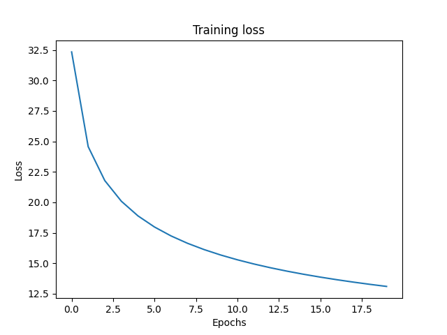
When running the following command python3.7 main.py --model lr the model is trained by the fit method and tested on the test dataset via the predict method.

Here is a picture of the loss during training. We can see that the loss nicely converges.

Thanks for taking the time to read all the way to the end.

Best, Hanna