By Group "Simplicity," written by Sean Uttsant RAI
Author Introduction
Hello, this is Sean. I'm a final year student studying Accounting and Finance at HKU, in charge of the correlation analysis portion of this project.
Overall Objective and Workflow
Using the processed data from the sentiment analysis portion, we need to compute the correlation between the sentiment values of the stocks discussed on the WallStreetBets subreddit and their respective stock returns. We have selected three different market shocks i.e. Crypto, COVID and GME and two random dates to use as anchors for our analysis. Then, we need to visualise and output the results across different timeframes i.e. 1 day, 1 week, 1 month, 3 month, 6 month, 1 year, for the chosen anchors to see whether the correlation values would change over time. The steps are shown below:
- Read the sentiment values CSV file as a DataFrame and convert the 'date' column to a yyyy-mm-dd format
- Create a list of lists of relevant stock tickers for the anchors i.e. 3 market shocks and 2 random dates
- Create main function that accepts input for timeframe i.e. number and interval e.g. 1 day/ 3 months, etc.
- Calculate the inputted timeframe's returns for stocks within the list of lists
- Calculate sentiment value average for relevant stocks depending on the timeframe inputed, and compute correlation
- Create a scatter plot for each anchor, where the x-axis: sentiment value average and y-axis: stock returns, and also add fitted line
- After repeating the above steps for all the timeframes, use list comprehension to plot the changes in correlation and p-value over time for all the anchors
Libraries and Modules Used:
import yfinance as yf
import pandas as pd
import scipy.stats as st
from datetime import datetime
from dateutil.relativedelta import relativedelta
import matplotlib.pyplot as plt
import seaborn as sns
import numpy as np
from numpy.polynomial.polynomial import polyfit
import os
1. Read the sentiment values CSV file as a DataFrame and convert the 'date' column to a yyyy-mm-dd format
save_path = r'/Users/uttsant/Desktop'
# CRYPTO, COVID, GME + 2 random dates
market_shocks = ['2018-09-20', '2020-02-20','2021-01-11', '2018-09-05', '2021-03-10']
# create dataframe for CSV with sentiment values
sentiment_csv_path = r'/Users/uttsant/Desktop/Updated_Data.csv'
df = pd.read_csv(sentiment_csv_path)
# convert date to yyyy-mm-dd format
df['date'] = df['date'].apply(lambda x: x.split()[0])
The values in the date column of the sentiment value CSV was in this format 2018-09-01 04:00:19+00:00. However the parameters for the yfinance function would require this format 2018-09-01. At first, I was think of using the datetime.strptime function to parse the string into the desired datetime format, and then use datetime.strftime function to convert it back to a string. However, I decided that using str.split and getting the first slice would be a lot more simpler and readable paired with the apply function for the df['date'] pandas series.
2. Create a list of lists of relevant stock tickers for the anchors i.e. 3 market shocks and 2 random dates
tickers_on_market_shocks = []
# create a list of tickers where the dates match the dates for the market shocks
for date in market_shocks:
    tickers_on_market_shocks.append(list(df[df['date'] == date].groupby('ticker').mean().index))
At first, I was struggling to retrieve the ticker values, because this code df[df['date'] == date].groupby('ticker').mean() would return a series for the mean, whereas I was interested in obtaining the ticker value. After looking up my issue online, I learnt that using the index attribute would return the ticker values that were the index in the series. I then converted it into a list, which was then appended to the tickers_on_market_shocks list, which formed a nested list.
3. Create main function that accepts input for timeframe i.e. number and interval e.g. 1 day/ 3 months, etc.
The first code block below is an excerpt of what I used as my old approach. All you need to know is that for every timeframe, in this case 1 day and 1 week, I would create a new block of basically the same code with a few variable names and values changed. Although the code could do its job and get the results I wanted, I realised that this approach would be very cumbersome to maintain, as a new block would have to be created every time a new timeframe was added and it could increase the risk of human error when updating the code, so it was definitely not a good practice.
#1 day return
full_one_day_return_df = pd.DataFrame()
labelled_one_day_return = pd.DataFrame()
one_day_return_list = []
for date in market_shock:
    start_date = datetime.strptime(date, '%Y-%m-%d') + relativedelta(days = 1)
    end_date = start_date + relativedelta(days = 1)
    for stock in ticker:
        temp_df = yf.download(stock, start = start_date, end = end_date, interval='1d')
        #calculate stock return and appending it to a list
        one_day_return_list.append((temp_df['Close'][-1] - temp_df['Close'][0])/ temp_df['Close'][0])
        full_one_day_return_df = full_one_day_return_df.append(temp_df)
labelled_one_day_return['Date and Tickers'] = labels
labelled_one_day_return['Return'] = one_day_return_list

#1 week return
full_one_week_return_df = pd.DataFrame()
labelled_one_week_return = pd.DataFrame()
one_week_return_list = []
for date in market_shock:
    start_date = datetime.strptime(date, '%Y-%m-%d') + relativedelta(days = 1)
    end_date = start_date + relativedelta(weeks = 1)
    for stock in ticker:
        temp_df = yf.download(stock, start = start_date, end = end_date, interval='1d')
        one_week_return_list.append((temp_df['Close'][-1] - temp_df['Close'][0])/ temp_df['Close'][0])
        full_one_week_return_df = full_one_week_return_df.append(temp_df)
labelled_one_week_return['Date and Tickers'] = labels
labelled_one_week_return['Return'] = one_week_return_list
So after racking my brain, I decided that using a self-defined function where the user can input the number and period to customise the timeframe, would be the way to go. I'll be referring to parts of this large block of code for the later steps as well. So do keep reading!
list_of_final_cs = []
list_of_returns = []
list_of_corr_p = []
def based_on_timeframe(number,period): #add 's' e.g. days, weeks, months, years
    #returns part
    zip_ = zip(market_shocks, tickers_on_market_shocks)
    for date, ticker_group in zip_:
        return_list = []
        ticker_list = []
        start_date = datetime.strptime(date, '%Y-%m-%d') + relativedelta(days = 1)
        if period == 'days':
            end_date = start_date + relativedelta(days = number)
        elif period == 'weeks':
            end_date = start_date + relativedelta(weeks = number)
        elif period == 'months':
            end_date = start_date + relativedelta(months = number)
        elif period == 'years':
            end_date = start_date + relativedelta(years = number)
        for ticker in ticker_group:
            try:
                temp_df = yf.download(ticker, start = start_date, end = end_date, interval='1d')
                return_list.append((temp_df['Close'][-1] - temp_df['Close'][0])/ temp_df['Close'][0])
                ticker_list.append(ticker + ' ' + date)

            except:
                pass
        list_of_returns.append(return_list)

        #sentiment value part
        if period == 'days':
            range_ = datetime.strptime(date, '%Y-%m-%d') + relativedelta(days = number)
        elif period == 'weeks':
            range_ = datetime.strptime(date, '%Y-%m-%d') + relativedelta(weeks = number)
        elif period == 'months':
            range_ = datetime.strptime(date, '%Y-%m-%d') + relativedelta(months = number)
        elif period == 'years':
            range_ = datetime.strptime(date, '%Y-%m-%d') + relativedelta(years = number)

        final_range = datetime.strftime(range_, '%Y-%m-%d')

        cs_average_series = df[(df['date'] >= date) & (df['date'] <= final_range)].groupby('ticker').mean()['Updated Score']

        relevant_tickers = []
        for i in ticker_list:
            if i.split()[1] == date:
                relevant_tickers.append(i.split()[0])

        final_cs = cs_average_series.loc[relevant_tickers]
        list_of_final_cs.append(list(final_cs))


        list_of_corr_p.append(st.pearsonr(list(final_cs),return_list))
        print(st.pearsonr(list(final_cs),return_list))

    #scatterplot for each market shock
    for i in range(len(list_of_final_cs)):
        plt.figure()

        x = np.array(list_of_final_cs[i])
        y = np.array(list_of_returns[i])
        b, m = polyfit(x, y, 1)
        plt.plot(x, y, '.')
        plt.plot(x, b + m * x, '-')

        plt.ylabel('WSB Sentiment Values')
        plt.xlabel('Stock Returns')
        plt.savefig(save_path + os.sep + str(i) + '.png')

    plt.show()

    #print correlation values and p-values for all the market shocks for this timeframe
    print(list_of_corr_p)
The first thing I did was create three empty lists. The lists are to store the sentiment values, returns, and correlation values & p-values for all the market_shocks inside the for-loop.
list_of_final_cs = []
list_of_returns = []
list_of_corr_p = []
4. Calculate the inputted timeframe's returns for stocks within the list of lists
def based_on_timeframe(number,period): #add 's' e.g. days, weeks, months, years
    #returns part
    zip_ = zip(market_shocks, tickers_on_market_shocks)
    for date, ticker_group in zip_:
        return_list = []
        ticker_list = []
        start_date = datetime.strptime(date, '%Y-%m-%d') + relativedelta(days = 1)
        if period == 'days':
            end_date = start_date + relativedelta(days = number)
        elif period == 'weeks':
            end_date = start_date + relativedelta(weeks = number)
        elif period == 'months':
            end_date = start_date + relativedelta(months = number)
        elif period == 'years':
            end_date = start_date + relativedelta(years = number)
        for ticker in ticker_group:
            try:
                temp_df = yf.download(ticker, start = start_date, end = end_date, interval='1d')
                return_list.append((temp_df['Close'][-1] - temp_df['Close'][0])/ temp_df['Close'][0])
                ticker_list.append(ticker + ' ' + date)
                # full_return_df = full_return_df.append(temp_df)

            except:
                pass
        list_of_returns.append(return_list)
When the for-loop for this part of the code is run, it is responsible for appending the returns for the stocks specified in the tickers_on_market_shocks list for all the market_shocks to the list_of_returns. Based on the number and period parameters that the user passes in the def based_on_timeframe(number,period): function, the end_date is assigned. For example, if based_on_timeframe(1, 'years') is inputted, the end_date will be exactly 1 year after the start_date. The start_date is automatically assigned depending on the market_shocks list's iterations. Also besides appending the returns, it also appends the ticker names + the date of the corresponding market shock to the ticker_list for later use.
5. Calculate sentiment value average for relevant stocks depending on the timeframe inputed, and compute correlation
#sentiment value part
if period == 'days':
    range_ = datetime.strptime(date, '%Y-%m-%d') + relativedelta(days = number)
elif period == 'weeks':
    range_ = datetime.strptime(date, '%Y-%m-%d') + relativedelta(weeks = number)
elif period == 'months':
    range_ = datetime.strptime(date, '%Y-%m-%d') + relativedelta(months = number)
elif period == 'years':
    range_ = datetime.strptime(date, '%Y-%m-%d') + relativedelta(years = number)

final_range = datetime.strftime(range_, '%Y-%m-%d')
This part of the code is for obtaining the date range for computing the sentiment value means. As stocks may be mentioned more than once within the selected timeframe. So for our analysis, we would need to compute the mean of the sentiment values for all the times they appeared on the subreddit within that timeframe. That's why we need to set a date range, which is decided based on the period parameter inputted.
sv_average_series = df[(df['date'] >= date) & (df['date'] <= final_range)].groupby('ticker').mean()['Updated Score']
This line of code finds the mean of the sentiment values for all the stocks that are included within the date range, and stores it as a pandas series for the Updated Score column.
relevant_tickers = []
for i in ticker_list:
    if i.split()[1] == date:
        relevant_tickers.append(i.split()[0])

final_sv = sv_average_series.loc[relevant_tickers]
list_of_final_sv.append(list(final_sv))
However, not all these stocks were mentioned on the subreddit during the actual market shocks. So we need to exclude the stocks that were not on the subreddit during the market shocks. In order to do that, we appended the ticker names that had dates that matched the market shock date, and appended to the relevant_tickers list. We then used the .loc function with the relevant_tickers list as an argument for the sv_average_series to obtain the sentiment value means for the relevant tickers.
list_of_corr_p.append(st.pearsonr(list(final_sv),return_list))
# print(st.pearsonr(list(final_sv),return_list))
This part of the code is responsible for computing the correlation values using the st.pearsonr function from the scipy.stats module, the final_sv series is converted to a list before being passed to the function, along with the return_list. The function returns both the correlation value and p-value inside a tuple. The tuples are appended to the list_of_corr_p list for plotting purposes in the final step.
6. Create a scatter plot for each anchor, where the x-axis: sentiment value average and y-axis: stock returns, and also add fitted line
As much as I wanted to integrate this part with the main for-loop instead of creating another for-loop, all the data points from the market shocks clump up together with the former approach, instead of being displayed separately, which was really frustrating. So, I had to resort to a separate for-loop which would run after the main for-loop ended.
for i in range(len(list_of_final_sv)):
        plt.figure()
        x = np.array(list_of_final_sv[i])
        y = np.array(list_of_returns[i])
        b, m = polyfit(x, y, 1)
        plt.plot(x, y, '.')
        plt.plot(x, b + m * x, '-')

        plt.ylabel('WSB Sentiment Values')
        plt.xlabel('Stock Returns')
        plt.savefig(save_path + os.sep + str(i) + '.png')

    plt.show()
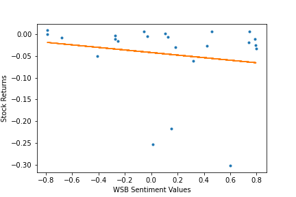
Here's an example of what the scatterplots would look like. This one is for the Crypto shock. It illustrates the relationship between the relevant stocks’ 1 day returns and their sentiment values over that 1 day after the crypto market shock.
7. Use list comprehension to plot the changes in correlation and p-value over time for all the anchors.
all_ is a three dimensional array, which contains all the correlation values and p-values that were computed in Step 5. The code below is for outputting the overall correlation trend across all timeframes for the Crypto shock. Initially, I planned on using a for-loop for this section, but I realised that it would look unnecessarily clunky. Then, I remembered about the list comprehension techniques we covered in a lecture. So, I used that to pass the values from all_ to crypto_corr and crypto_p for the line plots. The same was done for the rest of the shocks.
crypto_corr = [row[0][0] for row in all_]
crypto_p = [row[0][1] for row in all_]
x = ['1 day', '1 week', '1 month', '3 months', '6 months', '1 year']
sns.lineplot(x, crypto_corr, label = 'correlation value').set(title='Overall Correlation Trend for the Crypto Shock')
sns.lineplot(x, crypto_p, label = 'p-value')
Here is an overview of the overall correlation trend across all market shocks.
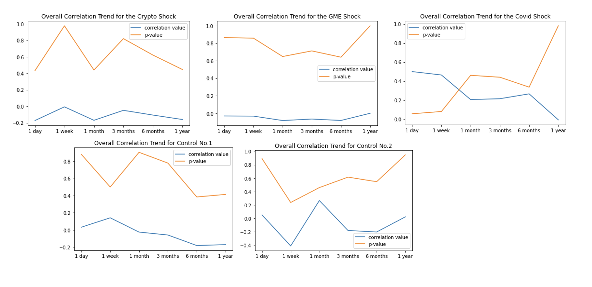
Final Thoughts
Generally speaking, the strength of the relationship between stock returns and sentiment values has remained weak throughout the 1 year period since the tested shocks. However, the consistently high p-values indicate that very little confidence should be placed in these relationships, since the probability of such a weak relationship due to random states is extremely high. Honestly speaking, the results were quite disappointing. I wasn't biased towards which side I wanted the correlation to lean towards, but I had at least hoped there would be reasonably low p-values, since it would have allowed us to make a more conclusive stance towards the subreddit's sentiments. But all in all, we still believe that our analysis can somewhat show that investing based on what WallStreetBets has to say would be a pretty huge gamble.