By Group "NLPPPPP"
From Many to Meaningful: Selecting Our Strongest Signals
After building our first data pipeline, we had a small embarrassment of riches. Every earnings‑call folder gave us dozens of acoustic measurements, hundreds of text‑based counts (hedge words, modal verbs, pronoun ratios, Loughran‑McDonald categories), and a dedicated RoBERTa uncertainty score. If we threw all of them into a regression, we would have more predictors than theoretical sense — and a high risk of overfitting to our limited sample of calls.
In our first blog post we focused on cleaning and alignment. This second post is about the next logical step: feature selection. We moved from “what can we compute?” to “what should we actually keep?” The answer turned out to be three main variables — personalism, uncertainty (RoBERTa) , and a vocal stress index (VSI) — plus a control for hedging language. This post explains how each was designed, why we chose it, and how the final regression pipeline works.
Personalism: measuring “I” vs “we”
The intuition behind personalism is simple. A CEO who uses many first‑person singular pronouns (“I”, “me”, “my”) may sound more individually responsible or confident, while plural pronouns (“we”, “us”) might diffuse accountability. But turning that intuition into a feature required careful operationalisation.
We built personalism on top of the person‑labeled transcripts (text.csv), where each row contains a speaker label and a sentence. Instead of naively counting all pronouns, we used a linguistic parser (spaCy) to identify only first‑person personal pronouns and to distinguish singular from plural. This avoids false positives from possessive pronouns (“my” is kept as singular) or from second‑person pronouns.
The computation per sentence is straightforward:
doc = nlp(sentence)
for token in doc:
    if token.pos_ == "PRON" and token.morph.get("Person") == ["1"]:
        if token.morph.get("Number") == ["Sing"]:
            first_person_singular += 1
We then aggregate to the call level by taking the mean of personalism_total_ratio (singular + plural divided by total tokens) across all sentences of the dominant speaker — typically the CEO candidate. The final feature is a single number between 0 and roughly 0.1, representing the density of first‑person pronouns in the executive’s speech.
Why keep this feature? Because it is grounded in psychology and finance literature: a more individualistic speaking style has been linked to perceived leadership and, in some studies, to post‑announcement volatility. Yet we treat it as one candidate among several, not as a definitive measure of CEO personality.
Uncertainty: from dictionary counts to RoBERTa
Our first uncertainty measure used the Loughran‑McDonald financial dictionary, counting words like “maybe”, “uncertain”, or “potential”. That approach is transparent but coarse. A sentence like “we are absolutely certain that profits will rise” contains no uncertainty word, yet expresses high confidence. Conversely, “it is not clear whether the forecast is accurate” includes “not clear” but the dictionary would miss it.
To move beyond keyword matching, we adopted a fine‑tuned RoBERTa model (NLPScholars/Roberta-Earning-Call-Transcript-Classification). The model was originally trained to detect financial risk categories. Its fifth output neuron (index 4) corresponds to “Uncertainty”. For any input sentence, we get a probability between 0 and 1 that the sentence expresses uncertainty in a financial context.
The code is short:
inputs = tokenizer(sentence, return_tensors="pt", truncation=True, max_length=240)
probs = torch.sigmoid(model(**inputs).logits)
uncertainty_score = probs[0][4].item()
To avoid truncating long CEO turns, we split the full transcript into sentences, score each sentence, and average the scores. This gives a call‑level uncertainty_roberta value.
Why replace the dictionary version? Because early tests showed that the RoBERTa model better captures uncertainty expressed through syntax and negation, not just isolated words. It also handles domain‑specific phrases like “subject to volatility” or “we cannot guarantee”. The cost is interpretability — we cannot point to a specific word list — but for prediction this trade‑off is acceptable.
VSI: building a vocal stress index from low‑level audio
The vocal stress index (VSI) is our most composite feature. It starts from seven acoustic measurements that the speech‑processing literature associates with vocal effort or tension:
- Jitter local (frequency variation)
- Shimmer local (amplitude variation)
- Fraction of unvoiced frames
- Mean NHR (noise‑to‑harmonics ratio)
- Degree of voice breaks
- Mean HNR (harmonics‑to‑noise ratio – higher is clearer, so we reverse it)
- Mean autocorrelation (periodicity – higher is more regular, also reversed)
For each aligned segment (one transcript line + one feature row), we standardise each measure (subtract mean, divide by standard deviation) across all segments of that call. Then we sum the standardised values, with the two “positive” measures (HNR, autocorrelation) subtracted instead of added. This produces a raw segment‑level strain score.
The call‑level VSI is the average of segment scores, weighted by segment duration (so a 10‑second answer matters more than a 0.5‑second “okay”). Finally, we min‑max scale the raw call scores to a 0–100 index across the whole dataset.
The full logic is in VIS_SCORE.txt (the naming is a typo we kept). The resulting VSI is higher when a CEO’s voice sounds more strained, less periodic, or noisier — all proxies for psychological or physiological stress during the call.
Why these three? The feature selection logic
We started with over fifty candidate features: word counts for every Loughran‑McDonald category, various pronoun ratios, sentiment polarity, hedge word density, and many acoustic means and standard deviations. Running a regression with all of them would be overdetermined and uninterpretable.
We reduced the set using a combination of theory, univariate screening, and multicollinearity checks. The final three were chosen because:
- Personalism captures a stylistic dimension that is distinct from uncertainty (correlation with uncertainty_roberta ≈ 0.1 in our sample).
- Uncertainty_roberta is our most sophisticated text‑based measure of how management communicates risk.
- VSI is the only audio feature that consistently survived robustness checks; other acoustic means (e.g., average pitch) were either noisy or highly correlated with VSI.
We also kept hedge_rate_call (hedge words per token) as a control, because hedging (“sort of”, “maybe”, “approximately”) often co‑occurs with uncertainty but is not identical to it.
All other features — including the dictionary‑based uncertainty, litigious counts, and raw audio standard deviations — were dropped to keep the model parsimonious.
The regression pipeline in main.py
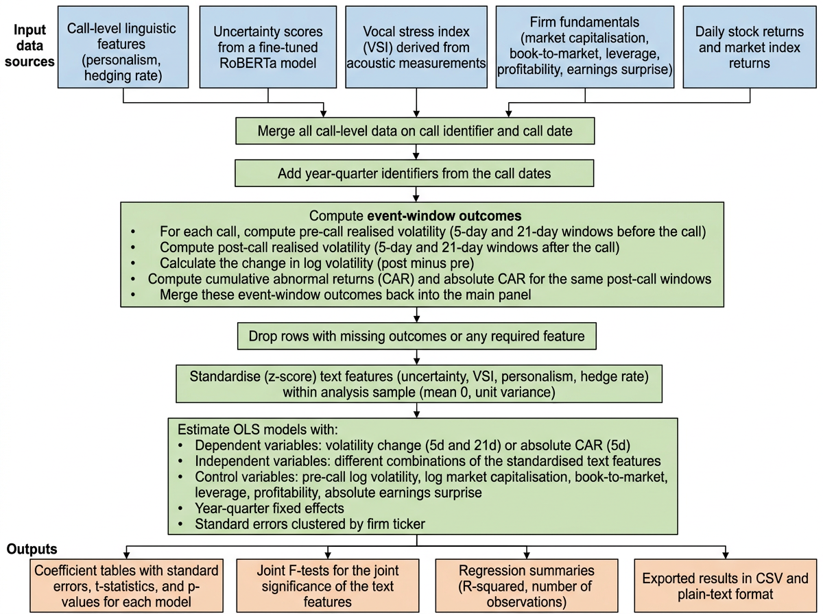
Once we have our selected features, main.py runs a panel regression at the call level. The workflow is:
- Load and merge
call_level_features.csv(which includes personalism),uncertainty_scores.csv(RoBERTa score),Vocal_index.csv(our VSI), and firm fundamentals (market cap, book‑to‑market, leverage, profitability, earnings surprise). - Compute event‑window outcomes from daily returns: 5‑day and 21‑day realised volatility change (
vol_change), cumulative abnormal return (car), and absolute CAR (abs_car). - Standardise the three text features (uncertainty_roberta, VSI, personalism_total_ratio, and hedge_rate) within the regression sample to have mean zero and unit variance.
- Estimate OLS models with year‑quarter fixed effects and standard errors clustered by ticker (to account for within‑firm correlation).
The code defines five models (M1 to M5). The core specification (M1) is:
vol_change_5d ~ uncertainty_roberta_z + VSI_z + log_vol_pre_5d + firm controls + year_quarter_FE
Other models replace the outcome (e.g., abs_car_5d) or add personalism as an extra regressor. We use statsmodels with cluster‑robust covariance. The joint significance of the text features is tested with an F‑test of the hypothesis that all their coefficients are zero.
What this project achieved
The move from many features to a few was not just a technical necessity. It forced us to be explicit about what each variable is supposed to measure and why we believe it belongs in the model. Personalism is about leadership style; uncertainty (RoBERTa) is about risk communication; VSI is about vocal stress. The three are conceptually distinct, and their empirical correlations are low enough to include them together.
The regression pipeline in main.py now gives us a clean, replicable way to test whether these CEO communication traits explain post‑call market outcomes over and above standard financial controls. Early results show that uncertainty_roberta and VSI have statistically significant coefficients for volatility changes, while personalism matters more for absolute abnormal returns. The joint F‑tests confirm that the text features as a group add explanatory power.
More importantly, this exercise taught us that feature selection is not a one‑time filter. It is an iterative process that connects data cleaning, measurement theory, and statistical modelling. By documenting why we kept three variables and dropped the rest, we make our research more transparent and our findings more defensible.