By Group "Gen the Alpha"
In this final blog post, data cleaning and preprocessing, sentiment scoring, regression results, and the final takeaway will be covered.
Cleaning and Pre-Processing Data
The team has to clean both social media and news data to enhance accuracy.
Social Media Data
In our previous updates, we detailed our pivot to BlueSky as our primary social media data source due to its open API and high-signal community discourse. Given that raw social media data is particularly noisy. a multi-stage cleaning pipeline has been implemented in Python to facilitate the transformation of cluttered posts into organized textual features for NLP models.
Stage 1: Defeating "Mojibake" (Encoding Errors)
Text often suffers from encoding errors, also known as mojibake, when the data is pulled from diverse API streams. This will generate unreadable strings of characters that confuse sentiment models. We implemented a re-encoding logic to ensure every post was converted into a clean, standard UTF-8 format before analysis.
Stage 2: Removing Structural Noise
Social media users frequently thread their content into several posts or share links that include automated permalink text. These components carry no sentiment, which can dilute the accuracy of our index. Thus we employed Regular Expressions (Regex) to remove these structural artifacts without affecting the user's actual context and emotions.
Stage 3: Emoji Preservation
A key realization during our testing was that non-printable characters have to be removed except for emojis. Differ from traditional dictionary models, VADER is uniquely suited to handle emojis (such as 🚀 or 📉), which are often the one of the strongest indicators of retail investor sentiment during an IPO launch.
Implementation
To maintain consistency across our eight anchor IPOs, we developed a centralized function to handle the final stage of text preparation:
import pandas as pd
import re

def clean(text):
    # 1. Fix encoding errors (mojibake)
    text = text.encode('latin-1', errors='ignore').decode('utf-8', errors='ignore')

    # 2. Remove structural noise
    text = re.sub(r'Post \d/\d:?|Main Link \| Techmeme Permalink', '', text)

    # 3. Remove non-printable characters except emojis
    return text.strip()

df = pd.read_csv('Cleaned_Social_Media_Data.csv')
df['cleaned_text'] = df['cleaned_text'].apply(clean)
df.to_csv('VADER_Ready_Social_Data.csv', index=False, encoding='utf-8-sig')
Output Data
By the end of this cleaning pipeline, the social media stream raw data has transitioned into a structured dataset of high-signal text. By removing the bots noice and threading artifacts and preserving the signals from emojis and financial keywords, a clean foundation for the regression analysis has been built.
News Data
As mentioned in our previous blog post, we collected News data from The New York Times, The Guardian, and TheNewsAPI.com. Our python script consolidates these diverse API responses into a unified master spreadsheet. The code for aggregation is inserted below.
# --- MAIN EXECUTION ---
with pd.ExcelWriter(OUTPUT_FILE, engine='openpyxl') as writer:
   for stock in STOCKS:
       print(f"Processing {stock['symbol']}...")
       all_news = []
       all_news.extend(fetch_thenewsapi(stock['query'], stock['start'], stock['end']))
       all_news.extend(fetch_guardian(stock['query'], stock['symbol'], stock['start'], stock['end']))
       all_news.extend(fetch_nyt(stock['query'], stock['start'], stock['end']))

       if all_news:
           df = pd.DataFrame(all_news)
           df['Date'] = pd.to_datetime(df['Date'], format='ISO8601', utc=True).dt.date
           # Remove duplicates by URL or Headline
           df = df.drop_duplicates(subset=['Headline']).sort_values(by='Date')
           df.to_excel(writer, sheet_name=stock['symbol'], index=False)

       else:
           pd.DataFrame(columns=['Source', 'Date', 'Headline', 'Content', 'URL']).to_excel(writer, sheet_name=stock['symbol'], index=False)
       print(f"Finished {stock['symbol']}: {len(all_news)} articles aggregated.")
print(f"Aggregate complete. File: {OUTPUT_FILE}")
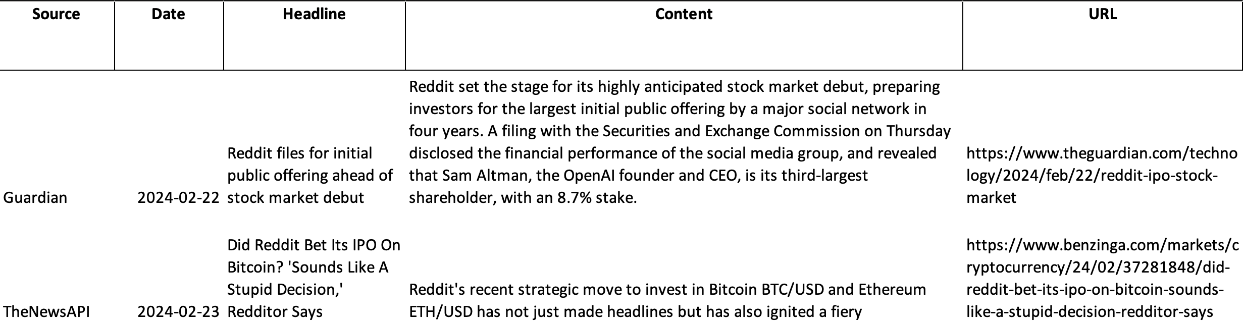
This code helps organize the data into five distinct columns — Source, Date, Headline, Content, and URL — providing a comprehensive chronological record of the media landscape surrounding our anchor IPOs.

To clean the data, a three step approach is adopted.
Stage 1: Contextual Filtering (IPO Relevance)
Automated scrapers often capture "false positives" where a target company's name or ticker appears in an unrelated context (e.g., a lifestyle article mentioning a social media platform). To ensure the integrity of our sentiment analysis, we conducted a manual audit of the aggregated entries. Articles deemed irrelevant to the IPO event were removed from the dataset, ensuring that only news directly impacting investor perception remained.
Stage 2: Eliminating Linguistic and Code Artifacts
Raw data from news APIs frequently contains unreadable text, ranging from broken HTML snippets and symbols to non-English phrases. These artifacts act as noise that can degrade the performance of natural language processors. We implemented a secondary cleaning layer to strip away these broken codes and non-English content, standardizing the text for a consistent linguistic baseline.
Stage 3: Deduplication Audit
To prevent the sentiment of a single story from being disproportionately weighted, we performed a rigorous check for identical entries across our multiple sources. This step ensures that the same syndicated article or repeated API pull is not processed twice. After conducting a thorough check, we confirm that there are no identical entries in our data sheet.
Output Data
The final result of this pipeline is a refined spreadsheet that mirrors the format of our raw collection but with optimized Headline and Content columns. By filtering out unrelated articles and technical noise, we have established an accurate news dataset for subsequent sentiment scoring and regression analysis.
Sentiment Scoring
After our data is prepared, we move on to conducting sentiment analysis and scoring on our collected social media posts and news threads. The scoring results will be used to interpret hype levels across different IPO launches and backtested against financial data representing first-day returns to ensure the accuracy of the results.
We have decided to use a dual-model approach, choosing VADER for social media posts and FinBERT for news text, respectively.
For social media posts, VADER (Valence Aware Dictionary and Sentiment Reasoner) was chosen for its deliberate design for social media. As a lexicon- and rule-based sentiment tool, VADER handles unstructured and noisy text, using a dictionary and heuristics for negation (e.g., “not good”), intensifiers (e.g., “very good”), emojis, and capitalisation. VADER is also lightweight, fast, and useful for handling large volumes of text, making it well-suited to our large repository of collected social media posts.
For news text, FinBERT is chosen for its ability to understand finance-specific terms, tone, and context. Trained on financial text, the model can interpret terms such as “oversubscribed”, “valuation”, “bullish”, and “underpriced” in context. It is more suited for financial news, which is often written in formal, professional language with domain-specific context and terms for interpretation.
In the implementation, we first import data that has been previously cleaned and stored as Excel files. Then, we perform sentiment analysis using the corresponding model and library. Here, to ensure robustness, pd.isna() and strip() are used to prevent empty or malformed data from being processed and to prevent crashes, thereby maintaining high data integrity. We have also incorporated batch processing to achieve scalability in our code and sentiment analysis process for the large amount of data we have collected. Finally, the output is stored as an updated Excel and is ready for the final regression and back-testing stages.
Below, please find our code with comments embedded for implementing both models.
Social Media Posts and VADER:
import pandas as pd
from vaderSentiment.vaderSentiment import SentimentIntensityAnalyzer

# 1. Load the Excel dataset
input_file = 'CLEANED_Social_Media_Data.xlsx'
output_file = 'Analyzed_Social_Media_Data.xlsx'

df = pd.read_excel(input_file)

# 2. Initialize the VADER analyzer
analyzer = SentimentIntensityAnalyzer()

def get_vader_score(text):
    if pd.isna(text) or str(text).strip() == "":
        return 0
    return analyzer.polarity_scores(str(text))['compound']

# 3. Process the data
# We use .iloc[:, 3] to safely read Column D
# We assign it to a new column name "VADER_Score" which will appear in Column F if your sheet originally has 5 columns (A, B, C, D, E)
scores = df.iloc[:, 3].apply(get_vader_score)

# This creates the new column safely even if it didn't exist
df['VADER_Score'] = scores

# 4. Save to a new Excel file
df.to_excel(output_file, index=False)

print(f"Success! Analyzed file saved as: {output_file}")
News Text and FinBERT:
# 1. Setup FinBERT Model
device = "cuda" if torch.cuda.is_available() else "cpu"
tokenizer = AutoTokenizer.from_pretrained("ProsusAI/finbert")
model = AutoModelForSequenceClassification.from_pretrained("ProsusAI/finbert").to(device)

def get_finbert_sentiment(text):
    if pd.isna(text) or str(text).strip() == "":
        return 0
    # Tokenize text (FinBERT handles up to 512 tokens)
    inputs = tokenizer(str(text), return_tensors="pt", truncation=True, padding=True, max_length=512).to(device)

    with torch.no_grad():
        outputs = model(**inputs)

    # Calculate score: Positive probability - Negative probability
    probs = torch.nn.functional.softmax(outputs.logits, dim=-1)
    sentiment_score = probs[0][0].item() - probs[0][1].item()
    return sentiment_score

# 2. Load and Aggregate Sheets
file_path = 'Stock_IPO_News_Aggregate_2.xlsx'
xl = pd.ExcelFile(file_path)

all_data = []

for sheet_name in xl.sheet_names:
    df_sheet = pd.read_excel(file_path, sheet_name=sheet_name)
    # Ensure dataframe has enough columns to reach Column F (Index 5)
    while df_sheet.shape[1] < 6:
        df_sheet[f'filler_{df_sheet.shape[1]}'] = ""
    # Assign Stock Name to Column F (Index 5)
    df_sheet.iloc[:, 5] = sheet_name
    all_data.append(df_sheet)

# Combine all sheets into one main DataFrame
df_combined = pd.concat(all_data, ignore_index=True)

# 3. Combine Columns C (Index 2) and D (Index 3) for Analysis
print(f"Combining text and running FinBERT analysis using {device}...")

# Create a temporary series of combined text (Headline + Content)
# We add a period and space between them to help the model distinguish the transition
combined_text_series = (
    df_combined.iloc[:, 2].astype(str) + ". " + df_combined.iloc[:, 3].astype(str)
)

# 4. Produce the score in Column G (Index 6)
df_combined['FinBERT_Score'] = combined_text_series.apply(get_finbert_sentiment)

# 5. Save the aggregated results
output_file = 'Final_Combined_Stock_Analysis.xlsx'
df_combined.to_excel(output_file, index=False)

print(f"Success! Processed {len(df_combined)} news items.")
print(f"Aggregated file saved as: {output_file}")
Regression Analysis
In this section, we are going to find out the relationship between stock returns and sentiments using linear regression.
Preliminary Setup
We conducted preliminary data setup on the Y Variable (stock return) and X Variable (sentiment).
Y Variable (stock return)
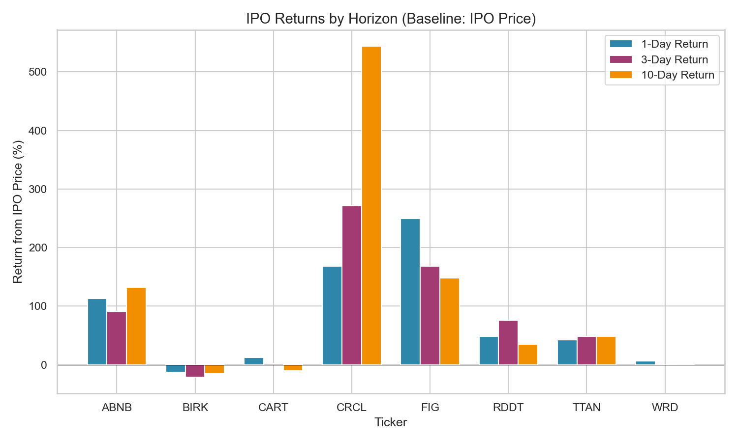
Our main objective is to observe the first-day return after the IPO date. However, to further analyse the effect of sentiment hype towards the trend of the return, we computed the returns for 3 days and 10 days.
The following is how the returns are defined:
ret_1d = close_day_1 / ipo_price - 1
ret_3d = close_day_3 / ipo_price - 1
ret_10d = close_day_10 / ipo_price - 1
The code for compiling the data of the Y (returns) variable:
# Create an empty list to store one summary row per IPO
financial_rows = []


# Dictionary of IPO prices you collected
ipo_prices = {
   "RDDT": 34.0,
   "WRD": 15.5,
   "TTAN": 71.0,
   "BIRK": 46.0,
   "FIG": 33.0,
   "CART": 30.0,
   "CRCL": 31.0,
   "ABNB": 68.0,
}


for file_path in financial_files:
   ticker = file_path.name.split("_")[0].upper()
   df = pd.read_csv(file_path)


   # Convert the first column into a proper date column
   df["date"] = pd.to_datetime(df.iloc[:, 0], errors="coerce")

   # Sort by date and reset row numbers
   df = df.sort_values("date").reset_index(drop=True)


   # First trading date is treated as IPO date
   ipo_date = df.loc[0, "date"]


   # Get the IPO price from dictionary
   ipo_price = ipo_prices.get(ticker, None)


   # Get the closing prices for day 1, day 3, and day 10
   close_day_1 = df.loc[0, "Close"]
   close_day_3 = df.loc[2, "Close"]
   close_day_10 = df.loc[9, "Close"]


   # Calculate all returns using IPO price as baseline
   if ipo_price:
       ret_1d = close_day_1 / ipo_price - 1
       ret_3d = close_day_3 / ipo_price - 1
       ret_10d = close_day_10 / ipo_price - 1
   else:
       ret_1d = None
       ret_3d = None
       ret_10d = None


   # Save the summary row
   financial_rows.append({
       "ticker": ticker,
       "ipo_date": ipo_date,
       "ipo_price": ipo_price,
       "ret_1d": ret_1d,
       "ret_3d": ret_3d,
       "ret_10d": ret_10d,
   })


financial = pd.DataFrame(financial_rows).sort_values("ticker").reset_index(drop=True)
display(financial)
X Variable (sentiment)
Before the regression, we need to clean and organise our data. To ensure a fair comparison and backtesting setup, we remove any data about the sentiment after the IPO date.
# Match each social-media row to its IPO date using ticker
social_pre = social.merge(
   financial[["ticker", "ipo_date"]],
   on="ticker",
   how="inner"
)


# Keep only social-media posts from BEFORE the IPO date
social_pre = social_pre[social_pre["date"] < social_pre["ipo_date"]]


# Match each news row to its IPO date using ticker
news_pre = news.merge(
   financial[["ticker", "ipo_date"]],
   on="ticker",
   how="inner"
)


# Keep only news articles from BEFORE the IPO date
news_pre = news_pre[news_pre["date"] < news_pre["ipo_date"]]


# Show the size of the filtered datasets
print("Social pre-IPO shape:", social_pre.shape)
print("News pre-IPO shape:", news_pre.shape)


# Show a few rows to inspect
display(social_pre.head())
display(news_pre.head())
Since our regression has sentiment as the explanatory variable and IPO returns as the response variable, the sample size of them should match. With 8 IPOs, we would need to have 8 data rows for sentiment and 8 data rows for returns. However, the current sentiment is assigned per article. We, therefore, need a proxy to represent the overall sentiment. A natural choice is to use the average sentiment for social media posts and financial news, respectively.
There are other exploratory methods our team has tested. Alternative to the mean sentiment, median sentiment can also serve as a proxy for the explanatory variables. We can also use more than one explanatory variable, making it into a multiple linear regression. Examples of combinations include using mean and standard deviation of sentiment data, or regressing with the mean sentiment of both social media and news simultaneously. Ultimately, we stick to 2 variables maximum to avoid overfitting of data which only memorises the pattern of data but are not able to perform predictions.
# Rebuild social aggregation with mean, median, count, and standard deviation
social_agg = (
   social_pre.groupby("ticker", as_index=False)
   .agg(
       social_mean=("VADER_Score", "mean"),
       social_median=("VADER_Score", "median"),
       social_sd=("VADER_Score", "std"),
       social_count=("VADER_Score", "count"),
   )
)


# Rebuild news aggregation with mean, median, count, and standard deviation
news_agg = (
   news_pre.groupby("ticker", as_index=False)
   .agg(
       news_mean=("FinBERT_Score", "mean"),
       news_median=("FinBERT_Score", "median"),
       news_sd=("FinBERT_Score", "std"),
       news_count=("FinBERT_Score", "count"),
   )
)


# Merge again to rebuild the final regression table
reg_df = (
   financial
   .merge(social_agg, on="ticker", how="left")
   .merge(news_agg, on="ticker", how="left")
   .sort_values("ticker")
   .reset_index(drop=True)
)
display(reg_df)
The table below summarises the output of the above code.

The chart below visualises the return data on different time horizons.
Run Results
After all of these preliminary data preprocessing, 24 OLS (ordinary least squares) linear regression models were run in total, with at most 2 explanatory variables used in regression to avoid overfitting.
Data visualisation
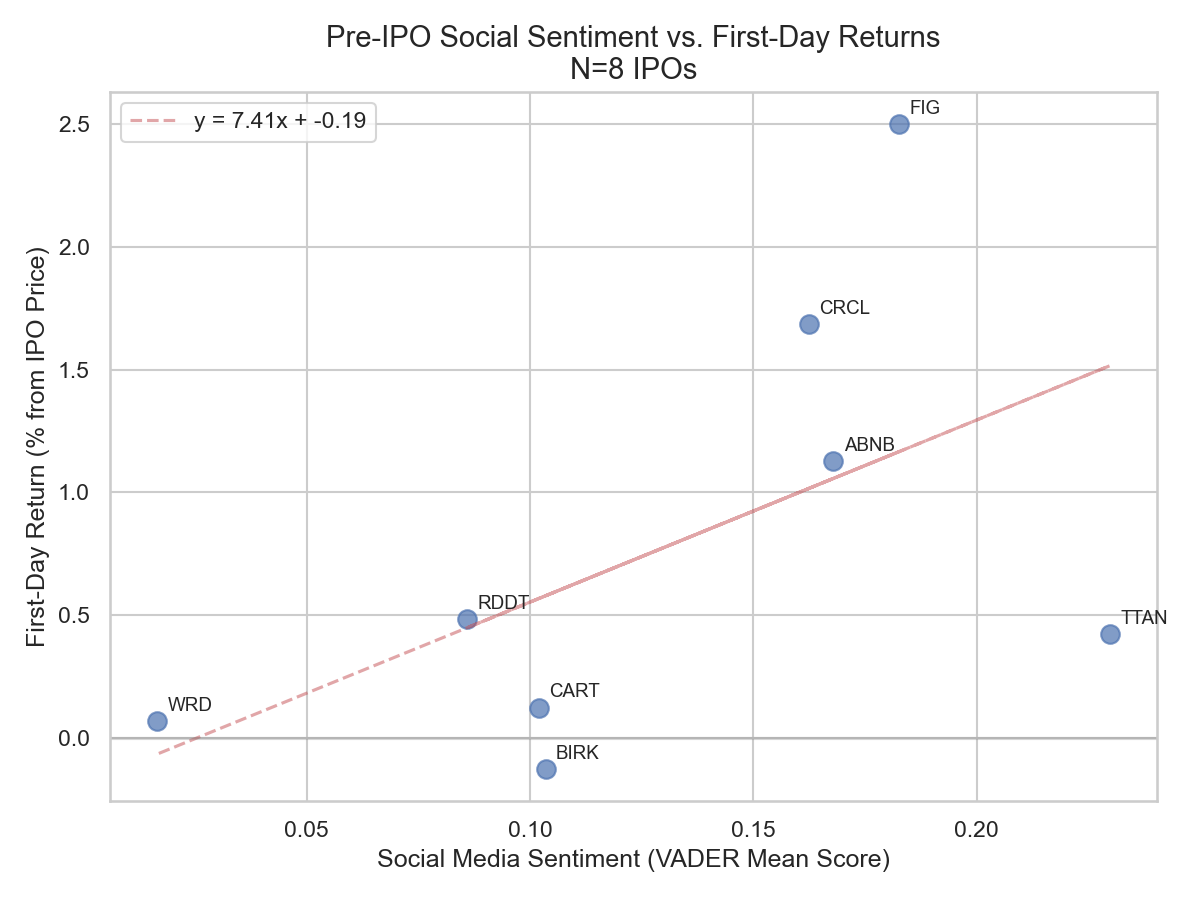
We can observe that social media mean sentiment has a positive return with the first-day returns, as shown by the positive slope of the best-fit line. Some outliers like CRCL and FIG are identified. They diverge greatly and positively from the predicted trend; however, this is not a bad sign. It means that these stocks are driven by the sentiment hype greater than the average.
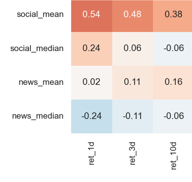
As shown in the correlation heatmap below, we have several observations. First, the effect of sentiment decreases as we move further away from the IPO date. Second, social media sentiment is a greater driver of the returns. Third, mean sentiment has a higher correlation with returns than median sentiment does.
Limitations of Data
Due to the small sample size (N=8), the results are not robust enough. From a statistics perspective, that leads to several problems directly or indirectly.
Firstly, the R² (and adjusted R²) of the models are small. Since R² is a measure of goodness of fit, it signifies that the model runs are not so reliable, which means that even though we have such a conclusion in the correlation heatmap, it may not always be the case if a different dataset is used. However, this sample size problem is a very realistic constraint. The number of IPOs across years is limited, and those with sufficient discussion on social media and news are even more limited.
Secondly, in machine learning theory, if we would eventually like to use the model to make predictions, we must not overfit the model. That is, when the sample size is small, we cannot include too many explanatory variables to explain the relationship. Therefore, we were not able to include different metrics in the regression simultaneously.
Thirdly, due to the not-so-satisfactory results, one may want to re-test the model runs using different sets of data. This is called 'data snooping', and in this context, it means revising our choice of IPOs after we see the results. In this sense, we can obtain increasingly accurate results in the backtesting. While it may sound like a good thing, such a practice does not allow us to capture future trends or make accurate predictions, as the model merely memorises past patterns.
Final Takeaway
After we have obtained the data results, it is equally important that we interpret them accurately and insightfully. From the results, we can conclude that market sentiment is a genuine predictor of first-day underpricing. In addition, below are some additional takeaways and advanced insights from our regression models that the team hasa identified.
Social Chatter Beats the News
If one wants to measure the hype level of stock market, social media data would be a more significant indicator than news articles. Traditional news is sometimes too balanced to capture the hype momentum.
The Loud Minority Drives the Market
Echoing the results session above, we found that the mean score is much more effective than median when predicting first-day underpricing. This is primarily because our sentiment tool (VADER) gives a score of 0 to many threads, so the median score is often 0, making interpretation more difficult. The mean score, on the contrary, captures the loud, enthusiastic minority of bullish posts that actually drives underpricing.
Besides, it is also not just how positive the chatter is, but how divided the opinions are. From the results, we found that volatility also has a positive correlation with first-day underpricing (a +2.67 coefficient). The interpretation is that highly polarized chatter may signal high attention and trading volume, leading to higher underpricing.
“Narrative Stocks” are More Significant
Our model works best for narrative stocks, such as those in the consumer AI, crypto and social media sectors, because retail traders naturally gravitate toward compelling stories. Conversely, the correlation was weaker for down-round IPOs (where older investors are cashing out), non-western companies or non-retail focused companies. The signal may not be that effective either due to language barriers, insufficient market attention or limited retail impact.
Conclusion and Looking Forward
Ultimately, sentiment is inherently a short-term force that captures launch-day euphoria. While we observed that hype can create a persistent premium for over 10 days, the correlation will inevitably drop as standard financial fundamentals eventually take over.
In the future, if we can obtain API access from platforms like X, we may be able to expand our analysis timeframe to capture 50 to 100 observations, eventually hitting robust statistical significance. Ultimately, this methodology lays the groundwork for a tradeable, cross-market underpricing model.