By Group "NLPPPPP"
Why our first week was about data, not prediction
When we gave our first presentation, our research question sounded elegant: can CEO communication style during earnings calls explain short-term market reactions beyond the numbers themselves? Our slide deck translated that idea into three candidate features—personalism, uncertainty, and vocal stress—and a later financial model built around realized volatility. That is the polished version of the project. The unpolished version, which is more appropriate for a first blog post, is that we spent our first serious week not doing "Fancy AI" but trying to make the raw data behave.
That turned out to be exactly the right place to begin.
The presentation framework is already ambitious. We want to use the MAEC earnings-call dataset for transcripts and low-level audio features, and later combine those call-level signals with market data and controls such as fundamentals and earnings surprise. The motivation is clear: investors may react not only to what management says, but also to how it is said. Boards may care because communication quality may have market value. Regulators may care because persuasive communication could move prices independently of fundamentals. All of that is interesting. But before any of those arguments can be tested, we need to answer a more basic question:
What exactly is one usable observation in this project?
That question became the center of our first-stage reflection.
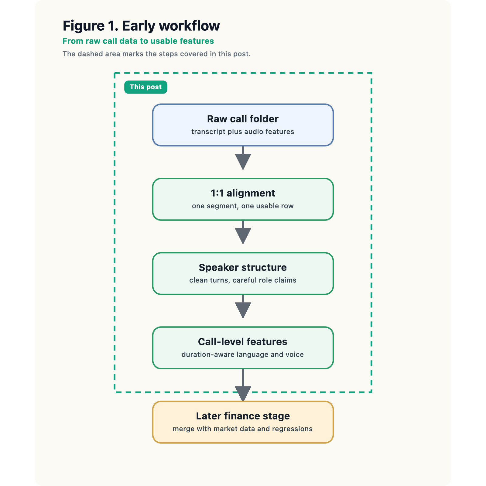
The first real problem: what counts as one observation?
At first glance, MAEC looks simple enough. In MAEC_Dataset, each earnings-call folder contains text.txt and features.csv. The transcript file stores one utterance per line, and the feature file stores one row of acoustic measurements per utterance. At the beginning, we treated this as a counting problem: if the number of transcript lines matched the number of feature rows, then maybe the data was “clean enough.”
That turned out to be too weak. In the course workflow, this is really a data-validation step: not just whether the counts match, but whether those two files can be turned into one aligned segment-level table that we can trust.
If the transcript were one giant document while the audio file were broken into many small segments, then a direct merge would be impossible. A call-level text score and a segment-level audio score do not live on the same observational level. That sounds like a minor data-wrangling nuisance, but in a multimodal project it is actually foundational. If the units do not match, any “voice-and-language” feature table is partly fiction.
So our first useful piece of code was not a model. It was a compact validation-and-construction step that checks one-to-one alignment and then makes the observational unit explicit.
from pathlib import Path
import pandas as pd

def build_segment_table(call_dir: str, preview_rows: int = 5) -> pd.DataFrame:
    call_path = Path(call_dir)
    text_path = call_path / "text.txt"
    feat_path = call_path / "features.csv"
    for p in (text_path, feat_path):
        if not p.is_file():
            raise FileNotFoundError(f"Expected file missing: {p.resolve()}")

    text_lines = [
        line.strip()
        for line in text_path.read_text(encoding="utf-8", errors="ignore").splitlines()
        if line.strip()
    ]
    audio_df = pd.read_csv(feat_path).reset_index(drop=True)
    audio_df.columns = audio_df.columns.str.strip()

    n_text, n_audio = len(text_lines), len(audio_df)
    if n_text != n_audio:
        raise ValueError(
            f"Alignment failed: {n_text} non-empty transcript lines vs "
            f"{n_audio} feature rows (units must match 1:1)."
        )

    text_df = pd.DataFrame({"segment_id": range(n_text), "text": text_lines})
    aligned = pd.concat([text_df, audio_df], axis=1)

    print(f"Segment-level table ({call_path.name})\n")
    print("  Each row = one transcript line + one acoustic feature row.")
    print(f"  Segments (observations): {n_text:,}")
    print(f"  Acoustic columns:        {len(audio_df.columns)}")
    print("  Alignment:               OK (1:1)")

    dur_col = "Audio Length"
    preview = aligned.head(preview_rows)
    show = {"segment_id": preview["segment_id"]}
    if dur_col in preview.columns:
        show["duration_s"] = pd.to_numeric(preview[dur_col], errors="coerce").round(2)
    for col in ("Mean pitch", "Mean intensity"):
        if col in preview.columns:
            key = "pitch_hz" if "pitch" in col.lower() else "intensity"
            show[key] = pd.to_numeric(preview[col], errors="coerce").round(2)
    preview_out = pd.DataFrame(show)

    if preview_rows > 0:
        print()
        print(f"First {preview_rows} segments (numeric preview only)\n")
        with pd.option_context("display.width", 120, "display.show_dimensions", False):
            print(preview_out.to_string(index=False))

    return aligned

segments = build_segment_table("MAEC_Dataset/20150226_ADSK")
Example run on call folder 20150226_ADSK:
- Each row = one transcript line + one acoustic feature row.
- Segments (observations): 60
- Acoustic columns: 29
- Alignment: OK (1:1)
First five segments (numeric preview only):
| segment_id | duration_s | pitch_hz | intensity |
|---|---|---|---|
| 0 | 1.69 | 501.21 | 29.33 |
| 1 | 5.29 | 143.61 | 59.70 |
| 2 | 9.61 | 124.76 | 53.61 |
| 3 | 1.79 | 140.12 | 32.01 |
| 4 | 0.37 | 160.70 | 53.29 |
What changed our understanding was not the equality check by itself. It was the realization that data validation here means making sure one line from text.txt and one row from features.csv can be combined into one usable multimodal observation. At first we thought alignment was mostly a counting problem. Then we realized it was a data-validation problem about the observational unit.
That matters because later feature engineering becomes much cleaner once the unit is explicit. We can compute text measures on each segment, keep acoustic measures on the same segment, and only then decide how to aggregate upward to the call level. In other words, the dataset becomes multimodal not because two files sit in one folder, but because they can be merged into one observation table without guessing.
Cleaner transcripts do not mean cleaner measurement
The next improvement came from looking at the person-labeled version of the dataset. In MAEC_Dataset_Person_Label, the transcript is no longer just raw lines in a text file. Instead, text.csv contains at least Person and Sentence, which means the conversation is already split into anonymous speaker turns.
In course-workflow terms, this sits in the cleaning / preprocessing stage. We can strip empty rows, standardize the sentence field, and inspect turn structure much more cleanly than before. But preprocessing the transcript does not automatically solve the harder measurement problem.
That was genuinely helpful, but it did not solve the problem we first hoped it would solve. The presence of a Person column tells us that the transcript has multi-speaker structure. It does not by itself tell us which speaker is the CEO, which one is an analyst, and which one is another manager. We realized pretty quickly that speaker separation is not the same as role separation.
So the second block of code became a preprocessing-and-inspection step for speaker structure rather than an overconfident “CEO language” measure.
def inspect_person_labeled_call(
    call_dir: str, preview_rows: int = 5, sentence_width: int = 70
) -> pd.DataFrame:
    df = pd.read_csv(Path(call_dir) / "text.csv")
    df["Sentence"] = df["Sentence"].fillna("").astype(str).str.strip()
    df = df[df["Sentence"] != ""].copy()
    df["word_count"] = df["Sentence"].str.split().str.len()

    turns = df["Person"].value_counts().sort_index()
    words = df.groupby("Person", sort=True)["word_count"].sum()
    summary = pd.DataFrame({"turns": turns, "words": words})
    summary["words/turn"] = (summary["words"] / summary["turns"]).round(1)
    summary.index.name = "speaker"
    total_turns = len(df)
    n_speakers = df["Person"].nunique()

    print(f"  Non-empty labelled turns: {total_turns:,}")
    print(f"  Distinct speakers:        {n_speakers}\n")
    print(summary.to_string())

    return df

speaker_df = inspect_person_labeled_call("MAEC_Dataset/20150226_ADSK")
Example run on call folder 20150226_ADSK:
- Non-empty labelled turns: 60
- Distinct speakers: 2
| speaker | turns | words | words/turn |
|---|---|---|---|
| Person0 | 49 | 708 | 14.4 |
| Person1 | 11 | 152 | 13.8 |
Even without assigning economic roles, this already tells us something important. We can see how many distinct speakers appear, who dominates the turn-taking, and how much text each anonymous speaker contributes. That is useful descriptive structure. But it still does not justify calling any early text metric a CEO-only variable.
This changed how we interpret our own prototype features. If we count pronouns, hedging words, or uncertainty language across all sentences in text.csv, we are probably measuring a mixed-speaker communication environment, not a clean CEO construct. A rise in “I” or “maybe” could come from the executive team, from analysts during Q&A, or from the interaction between them. That does not make the feature useless, but it changes what we are allowed to claim.
So section 2 became less about “cleaning noisy text” in a generic sense and more about measurement discipline. Cleaning and preprocessing help us see the structure of the transcript more clearly, but they do not remove speaker-role ambiguity. That was another small but important shift in our thinking.
Averaging is already a modeling decision
The presentation proposes a vocal stress index built from low-level audio features using Python, pandas, and numpy. Again, the idea sounds straightforward until we look closely at the structure of features.csv.
The file is not one row per call. It is one row per aligned segment.
In the course workflow, this is the data transformation / feature engineering step. We have to decide how many segment-level rows should become one call-level score. Should every segment get equal weight? Probably not. In our sample call, the shortest usable segment is about 0.2 seconds, the median is about 4.4 seconds, and the 95th percentile is about 14.4 seconds. If we average everything equally, a one-second acknowledgement could influence the final score as much as a much longer substantive answer.
That is not a statistical detail. It is a design decision.
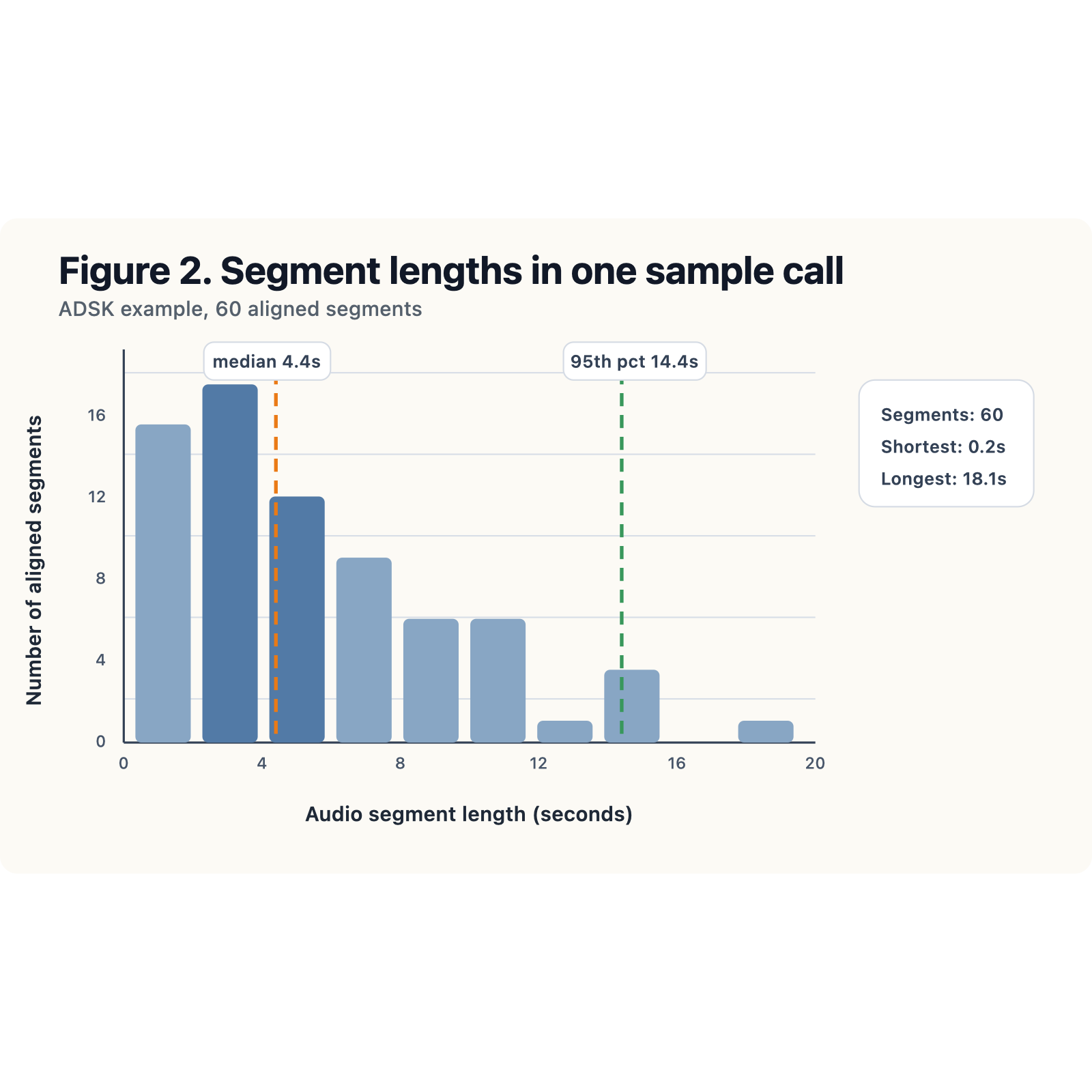
The histogram above made that issue visually obvious. Once we saw the spread in segment lengths, equal-weight averaging looked much harder to defend. That was a useful reminder that the workflow is iterative: the visualization was not decoration, it changed the aggregation choice.
So our prototype audio code treats aggregation as a transformation step, validates the key assumptions, and compares equal-weight and duration-weighted versions side by side.
import numpy as np
import pandas as pd

def vocal_stress_from_features(features_path: str, min_components: int = 3) -> dict:
    df = pd.read_csv(features_path)
    df.columns = df.columns.str.strip()

    audio_len_col = "Audio Length"
    # Higher values → more strain / less stable voice (literature-aligned).
    positive = [
        "Jitter local",
        "Shimmer local",
        "Fraction of unvoiced",
        "Mean NHR",
        "Degree of voice breaks",
    ]
    # Higher values → clearer / more periodic voice → subtract after z-scoring.
    negative = ["Mean HNR", "Mean autocorrelation"]
    feature_cols = positive + negative

    missing = [c for c in feature_cols + [audio_len_col] if c not in df.columns]
    if missing:
        raise KeyError(f"Missing columns: {missing}")

    raw = df[feature_cols + [audio_len_col]].apply(pd.to_numeric, errors="coerce")
    z_parts = []
    for c in positive:
        col = raw[c]
        mu, sig = col.mean(), col.std(ddof=0)
        z = (col - mu) / sig if sig and sig > 0 else pd.Series(0.0, index=col.index)
        z_parts.append(z.replace([np.inf, -np.inf], np.nan))

    for c in negative:
        col = raw[c]
        mu, sig = col.mean(), col.std(ddof=0)
        z = (col - mu) / sig if sig and sig > 0 else pd.Series(0.0, index=col.index)
        z_parts.append(-z.replace([np.inf, -np.inf], np.nan))

    Z = pd.concat(z_parts, axis=1, keys=feature_cols)
    counts = Z.notna().sum(axis=1)
    segment_score = Z.apply(lambda row: np.nanmean(row.values), axis=1)
    ok = (counts >= min_components) & raw[audio_len_col].notna()
    segment_score = segment_score.where(ok)
    weights = raw.loc[ok, audio_len_col].clip(lower=0.01)
    score = segment_score.loc[ok].dropna()

    if score.empty:
        raise ValueError("No segments with enough non-missing voice-quality features")

    out = {
        "segments_in_file": int(len(df)),
        "segments_scored": int(len(score)),
        "min_components_required": min_components,
        "vocal_strain_index_equal_weight": float(score.mean()),
        "vocal_strain_index_duration_weighted": float(np.average(score, weights=weights.loc[score.index])),
        "segment_strain_z": segment_score,
        "component_columns": feature_cols,
    }
    print(f"segments_in_file: {out['segments_in_file']}")
    print(f"segments_scored: {out['segments_scored']} (need ≥{min_components} of {len(feature_cols)} components)")
    print(f"vocal_strain_index (equal-weight over segments): {round(out['vocal_strain_index_equal_weight'], 4)}")
    print(f"vocal_strain_index (duration-weighted): {round(out['vocal_strain_index_duration_weighted'], 4)}")
    return out


audio_metrics = vocal_stress_from_features("MAEC_Dataset/20150226_ADSK/features.csv")
Example run on features.csv for 20150226_ADSK (minimum 3 of 7 components per segment):
| Metric | Value |
|---|---|
| Segments in file | 60 |
| Segments scored | 57 |
| Vocal strain index (equal-weight over segments) | -0.0079 |
| Vocal strain index (duration-weighted) | -0.0634 |
Even this simple prototype taught us two things. First, there can already be a small amount of numeric attrition after coercion and missing-value handling. Second, a call-level audio feature is never “just an average.” It depends on standardization, missing-data rules, weighting, and the theoretical direction assigned to each component.
At first aggregation looked like bookkeeping. Then we realized it was a transformation and design problem. In other words, feature engineering is already part of the research design, not a later add-on.
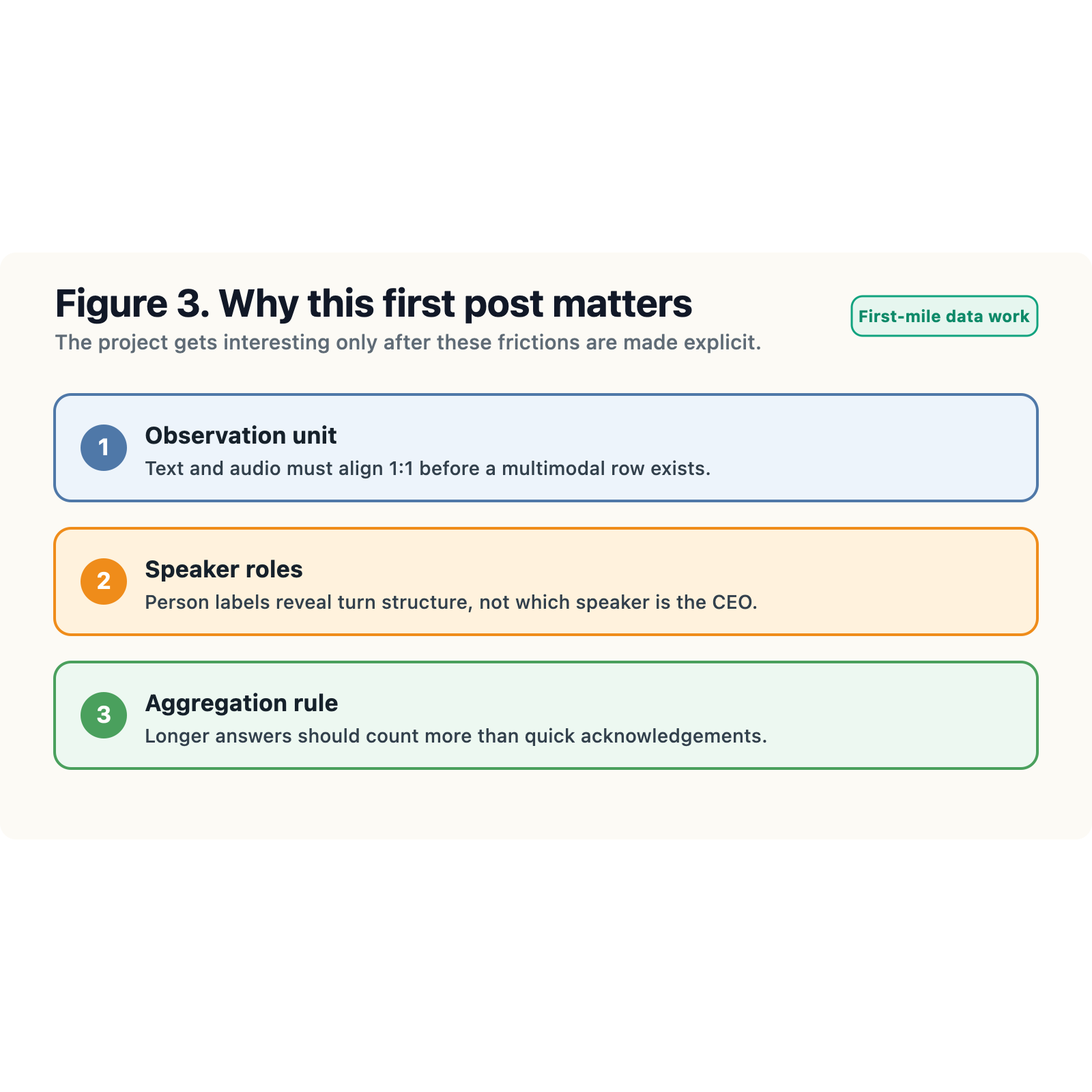
What this first stage was really about
Looking back, the most important progress we made this week was not building a final model. It was understanding how much of this project depends on careful preprocessing and a clear data workflow.
At the beginning, the project sounded quite clean: take earnings-call transcripts and audio features, build language and voice measures, and later connect them to market reactions. Once we opened the raw files, the work looked different. We had to:
- check whether text and audio were aligned at the same observational level;
- clarify what speaker labels did and did not tell us; and
- decide how segment-level features should become a call-level variable.
In that sense, this stage was less about prediction than about making the data usable.
That shift turned out to be valuable. Preprocessing is not just a routine step before the “real” analysis. Here, it already shapes the analysis: each decision about cleaning, alignment, and aggregation affects what our variables will mean later. This post is a reflection on how the project moved from a broad idea to a more structured workflow.
Where we go from here
The next step is to keep improving the preprocessing pipeline before moving on to the finance side. Concretely, we plan to:
- address speaker-role ambiguity more carefully;
- strengthen the text-side uncertainty measure; and
- make aggregation rules for the audio features more consistent and easier to justify.
Once these parts are clearer, we will be in a better position to build a cleaner call-level feature table and connect it to the later financial analysis.
At this stage, the clearest progress is in the workflow: how raw text and audio should be organized, how one usable observation should be defined, and why preprocessing decisions matter for everything that follows. With that foundation in place, the next step is to keep refining the pipeline and turn these early decisions into a more consistent feature set for the rest of the project.